Take-home Exercise 3

In this take-home exercise, I will build hedonic pricing models to explain factors affecting the resale prices of public housing in Singapore. The hedonic price models will be built by using appropriate GWR methods.

1. Background Information

• Housing is an essential component of household wealth worldwide.
• Buying a housing has always been a major investment for most people.
• The price of housing is affected by many factors.
  • Some of them are global in nature such as the general economy of a country or inflation rate.
  • Others can be more specific to the properties themselves.
    • These factors can be further divided to structural and locational factors.
• Structural factors are variables related to the property themselves such as the size, fitting, and tenure of the property.
• Locational factors are variables related to the neighbourhood of the properties such as proximity to childcare centre, public transport service and shopping centre.

Hedonic pricing model is used to examine the effect of housing factors as discussed above on the price.

• Conventional, this model was built by using Ordinary Least Square (OLS) method.
• However, this method failed to take into consideration that spatial autocorrelation and spatial heterogeneity exist in geographic data sets such as housing transactions.
• With the existence of spatial autocorrelation, the OLS estimation of hedonic pricing models could lead to biased, inconsistent, or inefficient results (Anselin 1998).
• In view of this limitation, Geographical Weighted Regression (GWR) was introduced for calibrating hedonic price model for housing.

2. Objective of analysis

In this take-home exercise, I will build hedonic pricing models to explain factors affecting the resale prices of public housing in Singapore. The hedonic price models will be built by using appropriate GWR methods.

3. Datasets

• Aspatial dataset:
  • HDB Resale data: a list of HDB resale transacted prices in Singapore from Jan 2017 onwards. It is in csv format which can be downloaded from Data.gov.sg.
• Geospatial dataset:
  • MP14_SUBZONE_WEB_PL: a polygon feature data providing information of URA 2014 Master Plan Planning Subzone boundary data. It is in ESRI shapefile format. This data set was also downloaded from Data.gov.sg
• Locational factors with geographic coordinates:
  • Downloaded from Data.gov.sg.
    • Eldercare data is a list of eldercare in Singapore. It is in shapefile format.
    • Hawker Centre data is a list of hawker centres in Singapore. It is in geojson format.
    • Parks data is a list of parks in Singapore. It is in geojson format.
    • Supermarket data is a list of supermarkets in Singapore. It is in geojson format.
    • CHAS clinics data is a list of CHAS clinics in Singapore. It is in geojson format.
    • Childcare service data is a list of childcare services in Singapore. It is in geojson format.
    • Kindergartens data is a list of kindergartens in Singapore. It is in geojson format.
  • Downloaded from Datamall.lta.gov.sg.
    • MRT data is a list of MRT/LRT stations in Singapore with the station names and codes. It is in shapefile format.
      
    • Bus stops data is a list of bus stops in Singapore. It is in shapefile format.
• Locational factors without geographic coordinates:
  • Downloaded from Data.gov.sg.
    • Primary school data is extracted from the list on General information of schools from data.gov portal. It is in csv format.
  • Retrieved/Scraped from other sources
    • CBD coordinates obtained from Google.
    • Shopping malls data is a list of Shopping malls in Singapore obtained from Wikipedia.
    • Good primary schools is a list of primary schools that are ordered in ranking in terms of popularity and this can be found at Local Salary Forum.

4. Install and Load R packages

This code chunk performs 3 tasks:

• A list called packages will be created and will consists of all the R packages required to accomplish this exercise.
• Check if R packages on package have been installed in R and if not, they will be installed.
• After all the R packages have been installed, they will be loaded.

packages <- c('sf', 'tidyverse', 'tmap', 'httr', 'jsonlite', 'rvest', 
              'sp', 'ggpubr', 'corrplot', 'broom',  'olsrr', 'spdep', 
              'GWmodel', 'devtools')
for(p in packages){
  if(!require(p, character.only = T)){
    install.packages(p)
  }
  library(p, character.only = T)
}

devtools::install_github("gadenbuie/xaringanExtra")
library(xaringanExtra)

More on the packages used:

• sf: used for importing, managing, and processing geospatial data

  • specifically vector-based geospatial data

• tidyverse: used for importing, wrangling and visualising data. It consists of a family of R packages, such as:

  • readr for importing csv data,
  • readxl for importing Excel worksheet,
  • tidyr for manipulating data,
  • dplyr for transforming data, and
  • ggplot2 for visualising data

• tmap: provides functions for plotting cartographic quality static point patterns maps or interactive maps by using leaflet API.

• httr: Useful tools for working with HTTP organised by HTTP verbs (GET(), POST(), etc). Configuration functions make it easy to control additional request components (authenticate(), add_headers() and so on).

  • In this analysis, it will be used to send GET requests to OneMapAPI SG to retrieve the coordinates of addresses.

• jsonlite: A simple and robust JSON parser and generator for R. It offers simple, flexible tools for working with JSON in R, and is particularly powerful for building pipelines and interacting with a web API.

• rvest: A new package that makes it easy to scrape (or harvest) data from html web pages, inspired by libraries like beautiful soup.

  • In this analysis, it will be used to scrape data for Shopping malls and Good primary schools

• sp: provides classes and methods for dealing with spatial data in R.

• ggpubr: provides some easy-to-use functions for creating and customizing ggplot2 based publication ready plots

  • In this analysis, it will be used to arrange multiple ggplots.

• corrplot: For Multivariate data visualisation and analysis

• broom: Takes the messy output of built-in functions in R, such as lm, nls, or t.test, and turns them into tidy tibble.

  • In this analysis, functions like tidy and glance will be used to construct a tibble / summmary of the model which is easier to look at.

• oslrr: Used to build OLD and performing diagnostic tests.

• spdep: For spatial dependence statistics.

• GWmodel: Calibrate geographical weighted family of modes.

• devtools: used for installing any R packages which is not available in RCRAN. In this exercise, I will be installing using devtools to install the package xaringanExtra which is still under development stage.

• xaringanExtra: is an enhancement of xaringan package. As it is still under development stage, we can still install the current version using install_github function of devtools. This package will be used to add Panelsets to contain both the r code chunk and results whereever applicable.

5. Importing and Wrangling of Aspatial data

• read_csv() function of readr package is used to import resale-flat-prices into R as a tibble data frame called resale
• glimpse() function of dplyr package is used to display the data structure

Code Chunk

resale <- read_csv("data/aspatial/resale-flat-prices.csv")

Glimpse

glimpse(resale)

When we load in the dataset for the first time, we can see that:

• The dataset contains 11 columns with 110,893 rows.
• The columns that are present in the data are: month, town, flat_type, block, street_name, storey_range, floor_area_sqm, flat_model, lease_commence_date, remaining_lease, resale_price.
• As we are only interested in four-room flat transactions during the transaction period from 1st January 2019 to 30th September 2020, we will be filtering this dataframe in the next part.

5.1 Filter resale data

Here, we use:

• filter() function of dplyr package to select our desired flat_type and dates store it in rs_subset
• unique() function of base R package to check whether flat_type and month have been extracted successfully

Code Chunk

rs_subset <-  filter(resale,flat_type == "4 ROOM") %>% 
              filter(month >= "2019-01" & month <= "2020-09")

Glimpse

glimpse(rs_subset)

Unique month

unique(rs_subset$month)

Unique flat_type

unique(rs_subset$flat_type)

From the results above, we can see that:

• From Jan 2019 to September 2020, there are 15901 transactions for four-room flat in Singapore.
• We have also correctly extracted the relevant month and flat_type.

5.2 Transform resale data

5.2.1 Create new columns

Here, we use mutate function of dplyr package to create columns such as:

• address: concatenation of the block and street_name columns using paste() function of base R package
• remaining_lease_yr & remaining_lease_mth: split the year and months part of the remaining_lease respectively using str_sub() function of stringr package then converting the character to integer using as.integer() function of base R package
• After performing mutate function, we will store the new data in rs_transform

Code Chunk

rs_transform <- rs_subset %>%
  mutate(rs_subset, address = paste(block,street_name)) %>%
  mutate(rs_subset, remaining_lease_yr = as.integer(str_sub(remaining_lease, 0, 2))) %>%
  mutate(rs_subset, remaining_lease_mth = as.integer(str_sub(remaining_lease, 9, 11)))

Head

head(rs_transform)

5.2.2 Sum up remaining lease in months

In the code chunk below, we will:

• Replace NA values in remaining_lease_mth with the value 0 with the help of is.na() function of base R package
• Multiply remaining_lease_yr by 12 to convert it to months unit
• Create remaining_lease_mths column using mutate function of dplyr package which contains the summation of the remaining_lease_yr and remaining_lease_mths using rowSums() function of base R package
• Select required columns for analysis using select() function of base R package

Code Chunk

rs_transform$remaining_lease_mth[is.na(rs_transform$remaining_lease_mth)] <- 0
rs_transform$remaining_lease_yr <- rs_transform$remaining_lease_yr * 12
rs_transform <- rs_transform %>% 
  mutate(rs_transform, remaining_lease_mths = rowSums(rs_transform[, c("remaining_lease_yr", "remaining_lease_mth")])) %>%
  select(month, town, address, block, street_name, flat_type, storey_range, floor_area_sqm, flat_model, 
         lease_commence_date, remaining_lease_mths, resale_price)

Head

head(rs_transform)

5.3 Retrieve Postal Codes and Coordinates of Addresses

This section will focus on retrieving the relevant data like postal codes and coordinates of the addresses which is required to get the proximity to locational factors later on.

5.3.1 Create a list storing unique addresses

• We create a list to store unique addresses to ensure that we do not run the GET request more than what is necessary
• We can also sort it to make it easier for us to see at which address the GET request will fail.
• Here, we use unique() function of base R package to extract the unique addresses then use sort() function of base R package to sort the unique vector.

add_list <- sort(unique(rs_transform$address))

5.3.2 Create function to retrieve coordinates from OneMap.Sg API

• 1. Firstly, we create a dataframe called postal_coords to store all the final retrieved coordinates
• 2. Secondly, we first use GET() function of httr package to make a GET request to https://developers.onemap.sg/commonapi/search
  • OneMap SG offers functions for us to query spatial data from the API in a tidy format and provides additional functionalities to allow easy data manipulation.
  • Here, we will be using their REST APIs to search address data for a given search value and retrieve the coordinates of the searched location.
  • The required variables to be included in the GET request is as follows:
    • searchVal: Keywords entered by user that is used to filter out the results.
    • returnGeom {Y/N}: Checks if user wants to return the geometry.
    • getAddrDetails {Y/N}: Checks if user wants to return address details for a point.
  • Note:
    • The JSON response returned will contain multiple fields.
    • However, we are only interested in the postal code and coordinates like Latitude & Longitude.
    • On their website, they also made an announcement on a minor text fix where they changed the word “LONGTITUDE” to “LONGITUDE” which we will be using the latter in this analysis.
• 3. We then create a dataframe new_row which will be used to store each final set of coordinates retrieved during the loop
• 4. We also need to check the number of responses returned and append to the main dataframe accordingly. This is because:
  • The no. of returned responses of the searched location, (indicated by variable found) , varies as some location might have only a single result while other locations might return multiple results.
    • For example, the address 2 JLN BATU returns 3 sets of postal codes and coordinates ( meaning found = 3).
    • Hence, what we can do is to first look at only those that does not have empty postal codes then take the first set/row of the coordinates
  • We can also check to see if the address is invalid by looking at the number of rows returned by request.
  • There will also be some addresses searched that are invalid. ( means found = 0)
  • This step was helpful in determining what was causing the error of the API Call. We will see in the later section what errors was caused by the invalid searched errors.
• 5. Lastly, we will append the returned response (new_row) with the necessary fields to the main dataframe (postal_coords) using rbind() function of base R package.

get_coords <- function(add_list){
  
  # Create a data frame to store all retrieved coordinates
  postal_coords <- data.frame()
    
  for (i in add_list){
    #print(i)

    r <- GET('https://developers.onemap.sg/commonapi/search?',
           query=list(searchVal=i,
                     returnGeom='Y',
                     getAddrDetails='Y'))
    data <- fromJSON(rawToChar(r$content))
    found <- data$found
    res <- data$results
    
    # Create a new data frame for each address
    new_row <- data.frame()
    
    # If single result, append 
    if (found == 1){
      postal <- res$POSTAL 
      lat <- res$LATITUDE
      lng <- res$LONGITUDE
      new_row <- data.frame(address= i, postal = postal, latitude = lat, longitude = lng)
    }
    
    # If multiple results, drop NIL and append top 1
    else if (found > 1){
      # Remove those with NIL as postal
      res_sub <- res[res$POSTAL != "NIL", ]
      
      # Set as NA first if no Postal
      if (nrow(res_sub) == 0) {
          new_row <- data.frame(address= i, postal = NA, latitude = NA, longitude = NA)
      }
      
      else{
        top1 <- head(res_sub, n = 1)
        postal <- top1$POSTAL 
        lat <- top1$LATITUDE
        lng <- top1$LONGITUDE
        new_row <- data.frame(address= i, postal = postal, latitude = lat, longitude = lng)
      }
    }

    else {
      new_row <- data.frame(address= i, postal = NA, latitude = NA, longitude = NA)
    }
    
    # Add the row
    postal_coords <- rbind(postal_coords, new_row)
  }
  return(postal_coords)
}

5.3.3 Call get_coords function to retrieve resale coordinates

coords <- get_coords(add_list)

5.3.4 Inspect results

• Here, we check whether the relevant columns contains any NA values with is.na() function of base R package and also “NIL”.

coords[(is.na(coords$postal) | is.na(coords$latitude) | is.na(coords$longitude) | coords$postal=="NIL"), ]

From the results above, we can see that:

• There are 2 addresses that does not contain any postal codes but contains the geographic coordinates:
  • 215 CHOA CHU KANG CTRL
  • 216 CHOA CHU KANG CTRL
  • When researched further, according to gothere.sg website, it seems like these 2 addresses have their respective postal codes:
    • 680215
    • 680216
  • However, as OneMapAPISG returned the same set of coordinates for both of these addresses, we shall proceed with keeping them as we are more interested in the coordinates for our analysis later on.
• Additionally, other addresses that contains the string “ST.GEORGE’S RD” have NA for the geographic coordinates.
  • With further testing, it seems like we have to change ST. GEORGE to SAINT GEORGE for OneMapAPISG to return the correct geographic coordinates for these addresses.
  • Hence, we will combine the successfully retrieved coordinates first and handle the invalid addresses separately.

5.3.5 Combine resale and coordinates data

• After retrieving the coordinates, we should combine the successful ones with our transformed resale dataset.
• We can do this using left_join() function of dplyr package and our data will be stored in rs_coords.

Code Chunk

rs_coords <- left_join(rs_transform, coords, by = c('address' = 'address'))

Head

head(rs_coords)

5.3.6 Handle invalid addresses

5.3.6.1 Replace sub string in invalid addresses in address column & extract to new DF

• sub() function of base R package is used to change ST. GEORGE to SAINT GEORGE
• grepl() function of base R package is used to extract rows with addresses containing SAINT GEORGE’S

Code Chunk

rs_coords$address <- sub("ST. GEORGE'S", "SAINT GEORGE'S", rs_coords$address)
rs_invalid <- rs_coords[grepl("SAINT GEORGE'S", rs_coords$address), ]

Glimpse

glimpse(rs_invalid)

From the results above, we can see that:

• There are 27 rows that contains “ST. GEORGE’S” as the street_name but has the substring replaced in the address column.

5.3.6.2 Create unique list of addresses again

add_list <- sort(unique(rs_invalid$address))

5.3.6.3 Call get_coords to retrieve resale coordinates again

rs_invalid_coords <- get_coords(add_list)

5.3.6.4 Inspect results again

• Here, we check whether the relevant columns contains any NA values with is.na() function of base R package.

rs_invalid_coords[(is.na(rs_invalid_coords$postal) | is.na(rs_invalid_coords$latitude) | is.na(rs_invalid_coords$longitude)), ]

5.3.6.5 Combine rs_invalid_coords with rs_coords data

• After retrieving the coordinates, we should combine it with our transformed resale dataset by performing a left join.
• We can do this using left_join() function of dplyr package.

Code Chunk

rs_coords_final <- rs_coords %>%
  left_join(rs_invalid_coords, by = c("address")) %>%
  mutate(latitude = ifelse(is.na(postal.x), postal.y, postal.x)) %>%
  mutate(latitude = ifelse(is.na(latitude.x), latitude.y, latitude.x)) %>%
  mutate(longitude = ifelse(is.na(longitude.x), longitude.y, longitude.x)) %>%
  select(-c(postal.x, latitude.x, longitude.x, postal.y, latitude.y, longitude.y))

Head

head(rs_coords_final)

5.5 Write file to rds

• As our subset resale dataset is now complete with the coordinates, we can now save it as an rds file.
• This also helps us to prevent running the GET request more than what is needed.

rs_coords_rds <- write_rds(rs_coords_final, "data/aspatial/rds/rs_coords.rds")

5.6 Read rs_coords RDS file

Code Chunk

rs_coords <- read_rds("data/aspatial/rds/rs_coords.rds")

Glimpse

glimpse(rs_coords)

5.6.1 Assign and Transform CRS and Check

• Since the coordinate columns are Latitude & Longitude which are in decimal degrees, the projected CRS will be WGS84.
• We will need to assign them the respective EPSG code 4326 first before transforming it to 3414 which is the EPSG code for SVY21.
• Here we use,
  • st_as_sf() function of sf package to convert the data frame into sf object
  • st_transform() function of sf package to transform the coordinates of the sf object

Code Chunk

rs_coords_sf <- st_as_sf(rs_coords,
                    coords = c("longitude", 
                               "latitude"),
                    crs=4326) %>%
  st_transform(crs = 3414)

st_crs

st_crs(rs_coords_sf)

5.6.2 Check for invalid geometries

length(which(st_is_valid(rs_coords_sf) == FALSE))

5.6.3 Plot hdb resale points

tmap_mode("view")
tm_shape(rs_coords_sf)+
  tm_dots(col="blue", size = 0.02)
tmap_mode("plot")

6. Import Locational Factors data

6.1 Locational Factors with geographic coordinates

6.1.1 Read and check CRS of Locational factors

Here we use,

• st_read of sf package to read simple features or layers from file
• st_crs of sf package to retrieve the coordinate reference system from sf object

Code Chunk

elder_sf <- st_read(dsn = "data/idptvar", layer="ELDERCARE")
mrtlrt_sf <- st_read(dsn = "data/idptvar", layer="MRTLRTStnPtt")
bus_sf <- st_read(dsn = "data/idptvar", layer="BusStop")

hawker_sf <- st_read("data/idptvar/hawker-centres-geojson.geojson") 
parks_sf <- st_read("data/idptvar/parks-geojson.geojson") 
supermkt_sf <- st_read("data/idptvar/supermarkets-geojson.geojson") 
chas_sf <- st_read("data/idptvar/chas-clinics-geojson.geojson")
childcare_sf <- st_read("data/idptvar/child-care-services-geojson.geojson") 
kind_sf <- st_read("data/idptvar/kindergartens-geojson.geojson") 

Check CRS

st_crs(elder_sf)
st_crs(mrtlrt_sf)
st_crs(bus_sf)
st_crs(hawker_sf)
st_crs(parks_sf)
st_crs(supermkt_sf)
st_crs(chas_sf)
st_crs(childcare_sf)
st_crs(kind_sf)

From the results above, we can see that:

• The datasets with WGS84 as the Geodetic CRS are:
  • childcare_sf, hawker_sf, kind_sf, parks_sf, supermkt_sf, chas_sf
  • As the EPSG code are in 4326 which is the appropriate EPSG code for WGS 84, we will only need to transform the CRS later on.
• While the datasets with SVY21 as the Projected CRS are:
  • elder_sf, mrtlrt_sf, busstop_sf
  • However, for all of these datasets, the EPSG code is 9001 which is wrong since the correct code for SVY21 should be 3414.

6.1.2 Assign EPSG code to sf dataframes and check again

Code Chunk

elder_sf <- st_set_crs(elder_sf, 3414)
mrtlrt_sf <- st_set_crs(mrtlrt_sf, 3414)
bus_sf <- st_set_crs(bus_sf, 3414)

hawker_sf <- hawker_sf %>%
  st_transform(crs = 3414)
parks_sf <- parks_sf %>%
  st_transform(crs = 3414)
supermkt_sf <- supermkt_sf %>%
  st_transform(crs = 3414)
chas_sf <- chas_sf %>%
  st_transform(crs = 3414)
childcare_sf <- childcare_sf %>%
  st_transform(crs = 3414)
kind_sf <- kind_sf %>%
  st_transform(crs = 3414)

Check CRS

st_crs(elder_sf)
st_crs(mrtlrt_sf)
st_crs(bus_sf)
st_crs(hawker_sf)
st_crs(parks_sf)
st_crs(supermkt_sf)
st_crs(chas_sf)
st_crs(childcare_sf)
st_crs(kind_sf)

From the above results, we can see that the EPSG code of all the data has now been assigned correctly and they are all EPSG 3414.

6.1.3 Check for invalid geometries

• Since the datasets above have the appropriate EPSG and the geometries, we should also check for any invalid geometries so that there won’t be any failure later on when we want to calculate the proximity or plot the map.
• Here, st_is_valid() of sf package is used to check for any invalid geometries.
• length() function of base R package is also used to get the count of invalid geometries if any.

length(which(st_is_valid(elder_sf) == FALSE))
length(which(st_is_valid(mrtlrt_sf) == FALSE))
length(which(st_is_valid(hawker_sf) == FALSE))
length(which(st_is_valid(parks_sf) == FALSE))
length(which(st_is_valid(supermkt_sf) == FALSE))
length(which(st_is_valid(chas_sf) == FALSE))
length(which(st_is_valid(childcare_sf) == FALSE))
length(which(st_is_valid(kind_sf) == FALSE))
length(which(st_is_valid(bus_sf) == FALSE))

From the results above, we can see that there are no invalid geometries for all of the locational factors.

6.1.4 Calculate Proximity

6.1.4.1 Create get_prox function to calculate proximity

• The following code chunk performs 3 steps:
  • 1. It will create a matrix of distances between the HDB and the locational factor using st_distance of sf package.
  • 2. It will also get the nearest point of the locational factor by looking at the minimum distance using min function of base R package then add it to HDB resale data under a new column using mutate() function of dpylr package.
  • 3. Lastly, it will rename the column name according to input given by user so that the columns have appropriate and distinct names that are different from one another.

get_prox <- function(origin_df, dest_df, col_name){
  
  # creates a matrix of distances
  dist_matrix <- st_distance(origin_df, dest_df)           
  
  # find the nearest location_factor and create new data frame
  near <- origin_df %>% 
    mutate(PROX = apply(dist_matrix, 1, function(x) min(x)) / 1000) 
  
  # rename column name according to input parameter
  names(near)[names(near) == 'PROX'] <- col_name

  # Return df
  return(near)
}

6.1.4.2 Call get_prox function

• Here, we call the get_prox function created earlier to get the proximity of the resale HDB and locational factors such as:
  • Eldercare
  • MRT
  • Hawker
  • Parks
  • Supermarkets
  • CHAS clinics
• The proximity will then be created as a new column under the rs_coords_sf dataframe.

rs_coords_sf <- get_prox(rs_coords_sf, elder_sf, "PROX_ELDERLYCARE") 
rs_coords_sf <- get_prox(rs_coords_sf, mrtlrt_sf, "PROX_MRT") 
rs_coords_sf <- get_prox(rs_coords_sf, hawker_sf, "PROX_HAWKER") 
rs_coords_sf <- get_prox(rs_coords_sf, parks_sf, "PROX_PARK") 
rs_coords_sf <- get_prox(rs_coords_sf, supermkt_sf, "PROX_SUPERMARKET")
rs_coords_sf <- get_prox(rs_coords_sf, chas_sf, "PROX_CHAS")

6.1.5 Create get_within function to calculate no. of factors within dist

• The following code chunk performs 3 steps:
  • 1. It will create a matrix of distances between the HDB and the locational factor using st_distance of sf package.
  • 2. It will also get the sum of points of the locational factor that are within the threshold distance using sum function of base R package then add it to HDB resale data under a new column using mutate() function of dpylr package.
  • 3. Lastly, it will rename the column name according to input given by user so that the columns have appropriate and distinct names that are different from one another.

get_within <- function(origin_df, dest_df, threshold_dist, col_name){
  
  # creates a matrix of distances
  dist_matrix <- st_distance(origin_df, dest_df)   
  
  # count the number of location_factors within threshold_dist and create new data frame
  wdist <- origin_df %>% 
    mutate(WITHIN_DT = apply(dist_matrix, 1, function(x) sum(x <= threshold_dist)))
  
  # rename column name according to input parameter
  names(wdist)[names(wdist) == 'WITHIN_DT'] <- col_name

  # Return df
  return(wdist)
}

6.1.5.1 Call get_within function

• Here, we call the get_within function created earlier to get the number of locational factors that are within a certain threshold distance.

• In this case, the threshold we set it to will be Within 350m for locational factors such as, Kindergartens, Childcare centres and Bus stops.

• Kindergarten

Code Chunk

rs_coords_sf <- get_within(rs_coords_sf, kind_sf, 350, "WITHIN_350M_KINDERGARTEN")

head

head(rs_coords_sf)

• Childcare centres

Code Chunk

rs_coords_sf <- get_within(rs_coords_sf, childcare_sf, 350, "WITHIN_350M_CHILDCARE")

head

head(rs_coords_sf)

• Bus stops

Code Chunk

rs_coords_sf <- get_within(rs_coords_sf, bus_sf, 350, "WITHIN_350M_BUS")

head

head(rs_coords_sf)

6.2 Locational Factors without geographic coordinates

In this section, we retrieve those locational factors that are not easily obtainable from data.gov.sg and/or does not have any geographic coordinates.

6.2.1 CBD

• So far, in our previous assignments, we know of the Planning Area called Downtown Core. However, this remains relatively unheard of by the public and the term Central Business District (CBD) is commonly used in conversation instead.
• Hence, with a quick Google search, the latitude and longitude of Downtown Core also known as CBD, are 1.287953 and 103.851784 respectively.
• As we already have the geographic coordinates of the resale data, we just need to convert the latitude and longitude of CBD area to EPSG 3414 (SVY21) format before we can run the get_prox function previously.
• We can first create a dataframe consisting of the latitude and longitude coordinates of the CBD area then transform it to EPSG 3414 (SVY21) format.

6.2.1.1 Store CBD coordinates in dataframe

name <- c('CBD Area')
latitude= c(1.287953)
longitude= c(103.851784)
cbd_coords <- data.frame(name, latitude, longitude)

6.2.1.2 Assign and Transform CRS

• Here we use,
  • st_as_sf() function of sf package to convert the data frame into sf object
  • st_transform() function of sf package to transform the coordinates of the sf object

Code Chunk

cbd_coords_sf <- st_as_sf(cbd_coords,
                    coords = c("longitude", 
                               "latitude"),
                    crs=4326) %>%
  st_transform(crs = 3414)

st_crs

st_crs(cbd_coords_sf)

• From the above results, we can see that the coordinates for CBD area in EPSG 3414 (SVY21) format is c(30055.05, 30040.83).
• Hence, we can now run our get_prox function to calculate the proximity of HDB and CBD area.

6.2.1.3 Call get_prox function

• Here, we call the get_prox function to get the proximity of HDB and CBD area.

rs_coords_sf <- get_prox(rs_coords_sf, cbd_coords_sf, "PROX_CBD") 

6.2.2 Shopping Malls

As there are currently no available datasets that we can download for Shopping Malls in Singapore, an alternative would be to extract the Shopping Mall names from Wikipedia and then get the respective coordinates with our get_coords function before computing the proximity.

6.2.2.1 Extract Shopping Malls from Wikipedia

• Since there are multiple lists of shopping malls classified by the regions in Singapore, we can check the XPaths of the various lists in the wikipedia page. The pattern identified here would be that the elements are unordered lists.
• The path expressions used in the following code chunk are:
  • [@attribute = 'value']: Select nodes with a particular attribute value
  • /: A beginning single slash indicates a select from the root node, subsequent slashes indicate selecting a child node from current node
  • text(): Select the text content of a node
  • This is something additional that I have learnt during my own time. It might take some time to get use to dealing with scraping from web pages, but once you get the basics down, it is very useful in getting the data you need.
  • You can read more about it at Library Carpentry
• In a nutshell, the following code chunk will perform 3 steps:
  • 1. Read the Wikipedia html page containing the Shopping Malls in Singapore
  • 2. Read the text portion (html_text()) of the Unordered List element selected by html_nodes()
  • 3. Append it to the empty mall_list created

Code Chunk

url <- "https://en.wikipedia.org/wiki/List_of_shopping_malls_in_Singapore"
malls_list <- list()

for (i in 2:7){
  malls <- read_html(url) %>%
    html_nodes(xpath = paste('//*[@id="mw-content-text"]/div[1]/div[',as.character(i),']/ul/li',sep="") ) %>%
    html_text()
  malls_list <- append(malls_list, malls)
}

st_crs

malls_list

From the results above, we can see that:

• There are about 169 shopping malls extracted.
• As these malls does not have the respective coordinates, we can use the get_coords function created previously to search the names of these shopping malls and retrieve them.

6.2.2.2 Call get_coords function

• We call the get_coords function to retrieve coordinates of Shopping Malls
• After calling the function, we will also rename the address to mall_name for easier reference

malls_list_coords <- get_coords(malls_list) %>% 
  rename("mall_name" = "address")

From the results above, we can see that:

• Some of the shopping mall names are not updated. For example,
  • POMO has been renamed to GR.ID
  • OD Mall has been renamed to The Grandstand
• Other shopping malls had minor issues where partial string of the Shopping Mall searched had successful responses.
  • For example,
    • Instead of searching Clarke Quay Central, searching Clarke Quay was good enough
    • Similarly, instead of searching City Gate Mall, searching City Gate was good enough
• Only one of the shopping mall, Yew Tee Shopping Centre, when researched further, was not existent.
  • Hence, we need to remove this row first.
• Also, in order for our analysis to be accurate as possible, we should fix all these issues first before moving forward.

6.2.2.3 Remove invalid Shopping Mall name

malls_list_coords <- subset(malls_list_coords, mall_name!= "Yew Tee Shopping Centre")

6.2.2.4 Correct invalid mall names that can be found

invalid_malls<- subset(malls_list_coords, is.na(malls_list_coords$postal))
invalid_malls_list <- unique(invalid_malls$mall_name)
corrected_malls <- c("Clarke Quay", "City Gate", "Raffles Holland V", "Knightsbridge", "Mustafa Centre", "GR.ID", "Shaw House",
                     "The Poiz Centre", "Velocity @ Novena Square", "Singapore Post Centre", "PLQ Mall", "KINEX", "The Grandstand")

for (i in 1:length(invalid_malls_list)) {
  malls_list_coords <- malls_list_coords %>% 
    mutate(mall_name = ifelse(as.character(mall_name) == invalid_malls_list[i], corrected_malls[i], as.character(mall_name)))
}

6.2.2.5 Create a list storing unique mall names

malls_list <- sort(unique(malls_list_coords$mall_name))

6.2.2.6 Call get_coords to retrieve coordinates of Shopping Malls again

malls_coords <- get_coords(malls_list)

6.2.2.7 Inspect results

• Here, we check whether the relevant columns contains any NA values with is.na() function of base R package.

malls_coords[(is.na(malls_coords$postal) | is.na(malls_coords$latitude) | is.na(malls_coords$longitude)), ]

6.2.2.8 Convert data frame into sf object, assign and transform CRS

• Here we use,
  • st_as_sf() function of sf package to convert the data frame into sf object
  • st_transform() function of sf package to transform the coordinates of the sf object

malls_sf <- st_as_sf(malls_coords,
                    coords = c("longitude", 
                               "latitude"),
                    crs=4326) %>%
  st_transform(crs = 3414)

6.2.2.9 Call get_prox function

• Here, we call the get prox function to get proximity of HDB and Shopping Malls

rs_coords_sf <- get_prox(rs_coords_sf, malls_sf, "PROX_MALL") 

6.2.3 Primary Schools

6.2.3.1 Read in CSV file

Code Chunk

pri_sch <- read_csv("data/idptvar/general-information-of-schools.csv")

Glimpse

glimpse(pri_sch)

6.2.3.2 Extract Primary Schools and required columns only

Code Chunk

pri_sch <- pri_sch %>%
  filter(mainlevel_code == "PRIMARY") %>%
  select(school_name, address, postal_code, mainlevel_code)

Glimpse

glimpse(pri_sch)

From the results above, we can see that there are 183 Primary Schools in Singapore.

6.2.3.3 Create list storing unique postal codes of Primary Schools

prisch_list <- sort(unique(pri_sch$postal_code))

6.2.3.4 Call get_coords function to retrieve coordinates of Primary Schools

prisch_coords <- get_coords(prisch_list)

6.2.3.5 Inspect results

• Here, we check whether the relevant columns contains any NA values with is.na() function of base R package.

prisch_coords[(is.na(prisch_coords$postal) | is.na(prisch_coords$latitude) | is.na(prisch_coords$longitude)), ]

6.2.3.6 Combine coordinates with Primary School Names

• Here, we combine the retrieved coordinates with the df that has the Primary School Names so that we can verify whether we have extracted it correctly.
• We combine it using the left_join function of dplyr package

Code Chunk

prisch_coords = prisch_coords[c("postal","latitude", "longitude")]
pri_sch <- left_join(pri_sch, prisch_coords, by = c('postal_code' = 'postal'))

Head

head(pri_sch)

6.2.3.7 Convert pri_sch data frame into sf object, assign and transform CRS

• Here we use,
  • st_as_sf() function of sf package to convert the data frame into sf object
  • st_transform() function of sf package to transform the coordinates of the sf object

Code Chunk

prisch_sf <- st_as_sf(pri_sch,
                    coords = c("longitude", 
                               "latitude"),
                    crs=4326) %>%
  st_transform(crs = 3414)

st_crs

st_crs(prisch_sf)

6.2.3.8 Call get_within function

• Here, we call the get_within function to get no. of Primary Schools within threshold of 1km or 1000m to be exact.

Code Chunk

rs_coords_sf <- get_within(rs_coords_sf, prisch_sf, 1000, "WITHIN_1KM_PRISCH")

Head

head(rs_coords_sf)

6.2.4 Good Primary Schools (Top 10)

• As there are no datasets that we can download from public data portals, an alternative would be to extract the “good” primary schools from forums or other websites.
• One particular forum that we can use is www.salary.sg where they provide a list of primary schools and rank them according to popularity.
• Similar to how we used XPath expression to scrape data for Shopping Malls in Singapore from Wikipedia, we will also use XPaths here.
• The difference is that here, the lists are ordered. Hence we have to change the ul to ol.
• Also the attribute is id instead.
  
• Salary SG Forum
• In a nutshell, the following code chunk will perform 4 steps:
  • 1. Read the Salary Forum html page containing the Good Primary Schools in Singapore
  • 2. Read all the text portion (html_text()) of the Ordered List element selected by html_nodes()
  • 3. Minor data transformation
    • Converting the name to uppercase
    • Deleting the substring in primary school names containg (PRIMARY SECTION)
    • Trim whitespaces
  • 4. Appending the schools extracted to a dataframe called good_pri and selecting the top 10 into top_good_pri dataframe

6.2.4.1 Extract Ranking List of Primary Schools

Code Chunk

url <- "https://www.salary.sg/2021/best-primary-schools-2021-by-popularity/"

good_pri <- data.frame()

schools <- read_html(url) %>%
  html_nodes(xpath = paste('//*[@id="post-3068"]/div[3]/div/div/ol/li') ) %>%
  html_text() 

for (i in (schools)){
  sch_name <- toupper(gsub(" – .*","",i))
  sch_name <- gsub("\\(PRIMARY SECTION)","",sch_name)
  sch_name <- trimws(sch_name)
  new_row <- data.frame(pri_sch_name=sch_name)
  # Add the row
  good_pri <- rbind(good_pri, new_row)
}

top_good_pri <- head(good_pri, 10)

Head

head(top_good_pri)

6.2.4.2 Check for good primary schools in primary school df

• As previously we have already retrieved the coordinates for primary schools, it would be good to reuse that dataframe to simply get the coordinates.
• However, before doing that, we need to check whether the names of the good primary schools is similar to the names in primary school dataframe using %in%

top_good_pri$pri_sch_name[!top_good_pri$pri_sch_name %in% prisch_sf$school_name]

Unfortunately, from the results above,

• There are 3 good primary schools that do not exist in the prisch_sf dataframe:
  • CATHOLIC HIGH SCHOOL
  • SAINT HILDA’S PRIMARY SCHOOL
  • CHIJ SAINT NICHOLAS GIRLS’ SCHOOL
• This is because, in the primary school data downloaded from data.gov.sg, these schools are classified as “MIXED LEVELS” under the mainlevel_code column.
• Hence, an alternative would be for us to just call the get_coords function

6.2.4.3 Create a list storing unique Good Primary School Names

good_pri_list <- unique(top_good_pri$pri_sch_name)

6.2.4.4 Call get_coords function to retrieve coordinates of Good Primary Schools

goodprisch_coords <- get_coords(good_pri_list)

6.2.4.5 Inspect results

• Here, we check whether the relevant columns contains any NA values with is.na() function of base R package.

goodprisch_coords[(is.na(goodprisch_coords$postal) | is.na(goodprisch_coords$latitude) | is.na(goodprisch_coords$longitude)), ]

From the results above, we can see that,

• There are 2 primary school that we are unable to retrieve the coordinates for:
  • CHIJ ST. NICHOLAS GIRLS’ SCHOOL
  • ST. HILDA’S PRIMARY SCHOOL
• With further research and testing, it is found that not only do we have to change the ST to SAINT, we also have to change the " ’ " used.

6.2.4.6 Replace invalid good primary school names

top_good_pri$pri_sch_name[top_good_pri$pri_sch_name == "CHIJ ST. NICHOLAS GIRLS’ SCHOOL"] <- "CHIJ SAINT NICHOLAS GIRLS' SCHOOL"
top_good_pri$pri_sch_name[top_good_pri$pri_sch_name == "ST. HILDA’S PRIMARY SCHOOL"] <- "SAINT HILDA'S PRIMARY SCHOOL"

6.2.4.7 Create a list storing unique Good Primary School Names again

good_pri_list <- unique(top_good_pri$pri_sch_name)

6.2.4.8 Call get_coords function to retrieve coordinates of Good Primary Schools again

goodprisch_coords <- get_coords(good_pri_list)

6.2.4.9 Inspect results again

• Here, we check whether the relevant columns contains any NA values with is.na() function of base R package.

goodprisch_coords[(is.na(goodprisch_coords$postal) | is.na(goodprisch_coords$latitude) | is.na(goodprisch_coords$longitude)), ]

From the results above, we can see that all the coordinates of the good primary schools have been retrieved successfully.

6.2.4.9 Convert data frame into sf objects, assign and transform CRS

• Here we use,
  • st_as_sf() function of sf package to convert the data frame into sf object
  • st_transform() function of sf package to transform the coordinates of the sf object

Code Chunk

goodpri_sf <- st_as_sf(goodprisch_coords,
                    coords = c("longitude", 
                               "latitude"),
                    crs=4326) %>%
  st_transform(crs = 3414)

st_crs

st_crs(goodpri_sf)

6.2.4.10 Call get_prox function

• Here, we call the get_prox function to get proximity of HDB and Good Primary Schools

rs_coords_sf <- get_prox(rs_coords_sf, goodpri_sf, "PROX_GOOD_PRISCH")

6.3 Write to RDS file

• As our subset resale dataset is now complete with all the locational factors, we can now save it as an rds file.
• This also helps us to prevent running the above codes.

rs_factors_rds <- write_rds(rs_coords_sf, "data/aspatial/rds/rs_factors.rds")

7. Import Data for Analysis

7.1 Geospatial data

Here we use,

• st_read of sf package to read simple features or layers from file
• st_crs of sf package to retrieve the coordinate reference system from sf object

7.1.1 MPSZ

Code Chunk

mpsz_sf <- st_read(dsn = "data/geospatial", layer="MP14_SUBZONE_WEB_PL")

Reading layer `MP14_SUBZONE_WEB_PL' from data source 
  `C:\aisyahajit2018\IS415\IS415_blog\_posts\2021-11-07-take-home-exercise-3\data\geospatial' 
  using driver `ESRI Shapefile'
Simple feature collection with 323 features and 15 fields
Geometry type: MULTIPOLYGON
Dimension:     XY
Bounding box:  xmin: 2667.538 ymin: 15748.72 xmax: 56396.44 ymax: 50256.33
Projected CRS: SVY21

st_crs

st_crs(mpsz_sf)

Coordinate Reference System:
  User input: SVY21 
  wkt:
PROJCRS["SVY21",
    BASEGEOGCRS["SVY21[WGS84]",
        DATUM["World Geodetic System 1984",
            ELLIPSOID["WGS 84",6378137,298.257223563,
                LENGTHUNIT["metre",1]],
            ID["EPSG",6326]],
        PRIMEM["Greenwich",0,
            ANGLEUNIT["Degree",0.0174532925199433]]],
    CONVERSION["unnamed",
        METHOD["Transverse Mercator",
            ID["EPSG",9807]],
        PARAMETER["Latitude of natural origin",1.36666666666667,
            ANGLEUNIT["Degree",0.0174532925199433],
            ID["EPSG",8801]],
        PARAMETER["Longitude of natural origin",103.833333333333,
            ANGLEUNIT["Degree",0.0174532925199433],
            ID["EPSG",8802]],
        PARAMETER["Scale factor at natural origin",1,
            SCALEUNIT["unity",1],
            ID["EPSG",8805]],
        PARAMETER["False easting",28001.642,
            LENGTHUNIT["metre",1],
            ID["EPSG",8806]],
        PARAMETER["False northing",38744.572,
            LENGTHUNIT["metre",1],
            ID["EPSG",8807]]],
    CS[Cartesian,2],
        AXIS["(E)",east,
            ORDER[1],
            LENGTHUNIT["metre",1,
                ID["EPSG",9001]]],
        AXIS["(N)",north,
            ORDER[2],
            LENGTHUNIT["metre",1,
                ID["EPSG",9001]]]]

Report above shows that:

• R object used to contain the imported MP14_SUBZONE_WEB_PL shapefile is called mpsz_sf and it is a simple feature object.
• The geometry type is multipolygon.
• It is also important to note that mpsz_sf simple feature object does not have EPSG information.
• The projected CRS for mpsz_sf** is also SVY21 but the EPSG code shown is 9001** which is wrong since the correct EPSG code for SVY21 should be 3414.

7.1.2 Transform CRS

Code Chunk

mpsz_sf <- st_transform(mpsz_sf, 3414)

st_crs

st_crs(mpsz_sf)

Coordinate Reference System:
  User input: EPSG:3414 
  wkt:
PROJCRS["SVY21 / Singapore TM",
    BASEGEOGCRS["SVY21",
        DATUM["SVY21",
            ELLIPSOID["WGS 84",6378137,298.257223563,
                LENGTHUNIT["metre",1]]],
        PRIMEM["Greenwich",0,
            ANGLEUNIT["degree",0.0174532925199433]],
        ID["EPSG",4757]],
    CONVERSION["Singapore Transverse Mercator",
        METHOD["Transverse Mercator",
            ID["EPSG",9807]],
        PARAMETER["Latitude of natural origin",1.36666666666667,
            ANGLEUNIT["degree",0.0174532925199433],
            ID["EPSG",8801]],
        PARAMETER["Longitude of natural origin",103.833333333333,
            ANGLEUNIT["degree",0.0174532925199433],
            ID["EPSG",8802]],
        PARAMETER["Scale factor at natural origin",1,
            SCALEUNIT["unity",1],
            ID["EPSG",8805]],
        PARAMETER["False easting",28001.642,
            LENGTHUNIT["metre",1],
            ID["EPSG",8806]],
        PARAMETER["False northing",38744.572,
            LENGTHUNIT["metre",1],
            ID["EPSG",8807]]],
    CS[Cartesian,2],
        AXIS["northing (N)",north,
            ORDER[1],
            LENGTHUNIT["metre",1]],
        AXIS["easting (E)",east,
            ORDER[2],
            LENGTHUNIT["metre",1]],
    USAGE[
        SCOPE["Cadastre, engineering survey, topographic mapping."],
        AREA["Singapore - onshore and offshore."],
        BBOX[1.13,103.59,1.47,104.07]],
    ID["EPSG",3414]]

7.1.3 Remove invalid geometries (if any)

7.1.3.1 Check for invalid geometries

• st_is_valid() is used to check for any invalid geometries.

length(which(st_is_valid(mpsz_sf) == FALSE))

[1] 9

7.1.3.2 Handle invalid geometries and check

• st_make_valid() to make the geometries valid for the mpsz_sf

mpsz_sf <- st_make_valid(mpsz_sf)
length(which(st_is_valid(mpsz_sf) == FALSE))

[1] 0

7.1.4 Reveal the extent of mpsz_sf

• Here, we reveal the extent of mpsz_sf using st_bbox() function of sf package

st_bbox(mpsz_sf)

     xmin      ymin      xmax      ymax 
 2667.538 15748.721 56396.440 50256.334 

7.2 Resale with locational factors

7.2.1 Read RDS file

Here we use:

• read_rds of readr package to read the previously saved rs_factors RDS file into rs_sf
• glimpse of dplyr package to see the transposed version of the dataframe

Code Chunk

rs_sf <- read_rds("data/aspatial/rds/rs_factors.rds")

Glimpse

glimpse(rs_sf)

Rows: 15,901
Columns: 26
$ month                    <chr> "2019-01", "2019-01", "2019-01", "2~
$ town                     <chr> "ANG MO KIO", "ANG MO KIO", "ANG MO~
$ address                  <chr> "204 ANG MO KIO AVE 3", "175 ANG MO~
$ block                    <chr> "204", "175", "543", "118", "411", ~
$ street_name              <chr> "ANG MO KIO AVE 3", "ANG MO KIO AVE~
$ flat_type                <chr> "4 ROOM", "4 ROOM", "4 ROOM", "4 RO~
$ storey_range             <chr> "01 TO 03", "07 TO 09", "01 TO 03",~
$ floor_area_sqm           <dbl> 92, 91, 92, 99, 92, 92, 92, 92, 93,~
$ flat_model               <chr> "New Generation", "New Generation",~
$ lease_commence_date      <dbl> 1977, 1981, 1981, 1978, 1979, 1981,~
$ remaining_lease_mths     <dbl> 684, 738, 733, 700, 715, 732, 706, ~
$ resale_price             <dbl> 330000, 360000, 370000, 375000, 380~
$ geometry                 <POINT [m]> POINT (29179.92 38822.08), PO~
$ PROX_ELDERLYCARE         <dbl> 0.2514065, 0.6318448, 1.0824168, 0.~
$ PROX_MRT                 <dbl> 0.6885144, 1.0969096, 0.8862859, 1.~
$ PROX_HAWKER              <dbl> 0.44182653, 0.26972560, 0.25829513,~
$ PROX_PARK                <dbl> 0.7450859, 0.4294870, 0.7800777, 0.~
$ PROX_SUPERMARKET         <dbl> 0.2708222, 0.3101889, 0.3187560, 0.~
$ PROX_CHAS                <dbl> 1.364596e-01, 2.569863e-01, 1.90618~
$ WITHIN_350M_KINDERGARTEN <int> 1, 1, 1, 1, 1, 1, 1, 1, 1, 0, 1, 1,~
$ WITHIN_350M_CHILDCARE    <int> 6, 5, 2, 3, 3, 2, 3, 4, 3, 2, 4, 4,~
$ WITHIN_350M_BUS          <int> 8, 8, 8, 7, 6, 9, 6, 6, 5, 4, 10, 5~
$ PROX_CBD                 <dbl> 8.824749, 9.841309, 9.560780, 9.609~
$ PROX_MALL                <dbl> 0.5534331, 1.0677012, 0.9751113, 1.~
$ WITHIN_1KM_PRISCH        <int> 2, 2, 1, 2, 2, 1, 3, 2, 2, 2, 2, 2,~
$ PROX_GOOD_PRISCH         <dbl> 1.2703931, 0.4045792, 2.0942375, 0.~

From the results above, we can see that:

• The data types of storey_range is in character type. This column can also be called a categorical variable.
• You might be thinking, Categorical variables..? In regression…?
• Yes, not all variables are the same.
• Categorical variables require special attention in regression analysis because, unlike continuous variables, they cannot be entered into the regression equation just as they are.
• Instead, they need to be recoded into a series of variables which can then be entered into the regression model.
  
• There are a variety of ways that we can recode categorical variables. A method most familiar to statisticians called “treatment” coding, which is another name for “dummy” coding where it consists of creating dichotomous variables where each level of the categorical variable is contrasted to a specified reference level.

But WAIT!

• Some categorical variables have levels that are ordered. Hence, they can be converted to numerical values instead and used as is.
• For example, there is some sort of a rank if we were to look at “Bad”, “Good” and “Excellent”.
• In our case, the storey_range also has a special meaning behind it if we were to order them from low to high.
• We might also get some insights as to whether resale prices are affected by storey range as units on the higher floors are generally said to offer more privacy, better security and hence a higher and better resale value.
• In the next section, instead of using dummy variables, we will be using sorting the storey_range categorical variable and assigning numerical values that are in ascending order.

7.2.2 Extract unique storey_range and sort

storeys <- sort(unique(rs_sf$storey_range))

7.2.3 Create dataframe storey_range_order to store order of storey_range

Code Chunk

storey_order <- 1:length(storeys)
storey_range_order <- data.frame(storeys, storey_order)

Head

head(storey_range_order)

   storeys storey_order
1 01 TO 03            1
2 04 TO 06            2
3 07 TO 09            3
4 10 TO 12            4
5 13 TO 15            5
6 16 TO 18            6

From the above results, we can see that:

• 01 TO 03 is assigned the value: 1
• 04 TO 06 is assigned the value: 2
• 07 TO 09 is assigned the value: 3

Hence, the storey range are in the correct order and is now in the correct type to be used for our regression model later on.

7.2.4 Combine storey_order with resale dataframe

Code Chunk

rs_sf <- left_join(rs_sf, storey_range_order, by= c("storey_range" = "storeys"))

Glimpse

glimpse(rs_sf)

Rows: 15,901
Columns: 27
$ month                    <chr> "2019-01", "2019-01", "2019-01", "2~
$ town                     <chr> "ANG MO KIO", "ANG MO KIO", "ANG MO~
$ address                  <chr> "204 ANG MO KIO AVE 3", "175 ANG MO~
$ block                    <chr> "204", "175", "543", "118", "411", ~
$ street_name              <chr> "ANG MO KIO AVE 3", "ANG MO KIO AVE~
$ flat_type                <chr> "4 ROOM", "4 ROOM", "4 ROOM", "4 RO~
$ storey_range             <chr> "01 TO 03", "07 TO 09", "01 TO 03",~
$ floor_area_sqm           <dbl> 92, 91, 92, 99, 92, 92, 92, 92, 93,~
$ flat_model               <chr> "New Generation", "New Generation",~
$ lease_commence_date      <dbl> 1977, 1981, 1981, 1978, 1979, 1981,~
$ remaining_lease_mths     <dbl> 684, 738, 733, 700, 715, 732, 706, ~
$ resale_price             <dbl> 330000, 360000, 370000, 375000, 380~
$ geometry                 <POINT [m]> POINT (29179.92 38822.08), PO~
$ PROX_ELDERLYCARE         <dbl> 0.2514065, 0.6318448, 1.0824168, 0.~
$ PROX_MRT                 <dbl> 0.6885144, 1.0969096, 0.8862859, 1.~
$ PROX_HAWKER              <dbl> 0.44182653, 0.26972560, 0.25829513,~
$ PROX_PARK                <dbl> 0.7450859, 0.4294870, 0.7800777, 0.~
$ PROX_SUPERMARKET         <dbl> 0.2708222, 0.3101889, 0.3187560, 0.~
$ PROX_CHAS                <dbl> 1.364596e-01, 2.569863e-01, 1.90618~
$ WITHIN_350M_KINDERGARTEN <int> 1, 1, 1, 1, 1, 1, 1, 1, 1, 0, 1, 1,~
$ WITHIN_350M_CHILDCARE    <int> 6, 5, 2, 3, 3, 2, 3, 4, 3, 2, 4, 4,~
$ WITHIN_350M_BUS          <int> 8, 8, 8, 7, 6, 9, 6, 6, 5, 4, 10, 5~
$ PROX_CBD                 <dbl> 8.824749, 9.841309, 9.560780, 9.609~
$ PROX_MALL                <dbl> 0.5534331, 1.0677012, 0.9751113, 1.~
$ WITHIN_1KM_PRISCH        <int> 2, 2, 1, 2, 2, 1, 3, 2, 2, 2, 2, 2,~
$ PROX_GOOD_PRISCH         <dbl> 1.2703931, 0.4045792, 2.0942375, 0.~
$ storey_order             <int> 1, 3, 1, 2, 2, 4, 3, 2, 4, 3, 3, 3,~

7.2.5 Select required columns for analysis

Code Chunk

rs_req <- rs_sf %>%
  select(resale_price, floor_area_sqm, storey_order, remaining_lease_mths,
         PROX_CBD, PROX_ELDERLYCARE, PROX_HAWKER, PROX_MRT, PROX_PARK, PROX_GOOD_PRISCH, PROX_MALL, PROX_CHAS,
         PROX_SUPERMARKET, WITHIN_350M_KINDERGARTEN, WITHIN_350M_CHILDCARE, WITHIN_350M_BUS, WITHIN_1KM_PRISCH)

Glimpse

glimpse(rs_req)

Rows: 15,901
Columns: 18
$ resale_price             <dbl> 330000, 360000, 370000, 375000, 380~
$ floor_area_sqm           <dbl> 92, 91, 92, 99, 92, 92, 92, 92, 93,~
$ storey_order             <int> 1, 3, 1, 2, 2, 4, 3, 2, 4, 3, 3, 3,~
$ remaining_lease_mths     <dbl> 684, 738, 733, 700, 715, 732, 706, ~
$ PROX_CBD                 <dbl> 8.824749, 9.841309, 9.560780, 9.609~
$ PROX_ELDERLYCARE         <dbl> 0.2514065, 0.6318448, 1.0824168, 0.~
$ PROX_HAWKER              <dbl> 0.44182653, 0.26972560, 0.25829513,~
$ PROX_MRT                 <dbl> 0.6885144, 1.0969096, 0.8862859, 1.~
$ PROX_PARK                <dbl> 0.7450859, 0.4294870, 0.7800777, 0.~
$ PROX_GOOD_PRISCH         <dbl> 1.2703931, 0.4045792, 2.0942375, 0.~
$ PROX_MALL                <dbl> 0.5534331, 1.0677012, 0.9751113, 1.~
$ PROX_CHAS                <dbl> 1.364596e-01, 2.569863e-01, 1.90618~
$ PROX_SUPERMARKET         <dbl> 0.2708222, 0.3101889, 0.3187560, 0.~
$ WITHIN_350M_KINDERGARTEN <int> 1, 1, 1, 1, 1, 1, 1, 1, 1, 0, 1, 1,~
$ WITHIN_350M_CHILDCARE    <int> 6, 5, 2, 3, 3, 2, 3, 4, 3, 2, 4, 4,~
$ WITHIN_350M_BUS          <int> 8, 8, 8, 7, 6, 9, 6, 6, 5, 4, 10, 5~
$ WITHIN_1KM_PRISCH        <int> 2, 2, 1, 2, 2, 1, 3, 2, 2, 2, 2, 2,~
$ geometry                 <POINT [m]> POINT (29179.92 38822.08), PO~

7.2.6 View summary

• Here we use summary() function of base R package to see the 5 number summaries of the numeric columns in rs_coords_sf

summary(rs_req)

  resale_price     floor_area_sqm    storey_order   
 Min.   : 218000   Min.   : 74.00   Min.   : 1.000  
 1st Qu.: 353000   1st Qu.: 91.00   1st Qu.: 2.000  
 Median : 405000   Median : 93.00   Median : 3.000  
 Mean   : 433589   Mean   : 95.15   Mean   : 3.258  
 3rd Qu.: 470000   3rd Qu.:102.00   3rd Qu.: 4.000  
 Max.   :1186888   Max.   :138.00   Max.   :17.000  
 remaining_lease_mths    PROX_CBD       PROX_ELDERLYCARE
 Min.   : 546.0       Min.   : 0.9994   Min.   :0.0000  
 1st Qu.: 798.0       1st Qu.:10.1651   1st Qu.:0.3017  
 Median : 936.0       Median :13.4356   Median :0.6251  
 Mean   : 939.8       Mean   :12.5368   Mean   :0.8084  
 3rd Qu.:1111.0       3rd Qu.:15.4162   3rd Qu.:1.1486  
 Max.   :1164.0       Max.   :19.6501   Max.   :3.3016  
  PROX_HAWKER         PROX_MRT         PROX_PARK      
 Min.   :0.03334   Min.   :0.02204   Min.   :0.04416  
 1st Qu.:0.38031   1st Qu.:0.30141   1st Qu.:0.51082  
 Median :0.65925   Median :0.53671   Median :0.72476  
 Mean   :0.76430   Mean   :0.60983   Mean   :0.82681  
 3rd Qu.:0.97793   3rd Qu.:0.82722   3rd Qu.:1.04233  
 Max.   :2.86763   Max.   :2.13061   Max.   :2.41314  
 PROX_GOOD_PRISCH     PROX_MALL        PROX_CHAS     
 Min.   : 0.06525   Min.   :0.0000   Min.   :0.0000  
 1st Qu.: 2.27448   1st Qu.:0.3690   1st Qu.:0.1152  
 Median : 4.01547   Median :0.5701   Median :0.1782  
 Mean   : 4.18757   Mean   :0.6358   Mean   :0.1925  
 3rd Qu.: 5.77804   3rd Qu.:0.8319   3rd Qu.:0.2509  
 Max.   :10.62237   Max.   :2.2710   Max.   :0.8083  
 PROX_SUPERMARKET    WITHIN_350M_KINDERGARTEN WITHIN_350M_CHILDCARE
 Min.   :0.0000001   Min.   :0.000            Min.   : 0.000       
 1st Qu.:0.1721851   1st Qu.:0.000            1st Qu.: 3.000       
 Median :0.2589783   Median :1.000            Median : 4.000       
 Mean   :0.2831776   Mean   :1.011            Mean   : 3.879       
 3rd Qu.:0.3660901   3rd Qu.:1.000            3rd Qu.: 5.000       
 Max.   :1.5713170   Max.   :7.000            Max.   :20.000       
 WITHIN_350M_BUS  WITHIN_1KM_PRISCH          geometry    
 Min.   : 0.000   Min.   :0.000     POINT        :15901  
 1st Qu.: 6.000   1st Qu.:2.000     epsg:3414    :    0  
 Median : 8.000   Median :3.000     +proj=tmer...:    0  
 Mean   : 7.982   Mean   :3.276                          
 3rd Qu.:10.000   3rd Qu.:4.000                          
 Max.   :18.000   Max.   :9.000                          

8. Exploratory Data Analysis

8.1 EDA using statistical graphics

8.1.1 Plot Histogram of resale_price

ggplot(data=rs_req, aes(x=`resale_price`)) +
  geom_histogram(bins=20, color="black", fill="light coral")

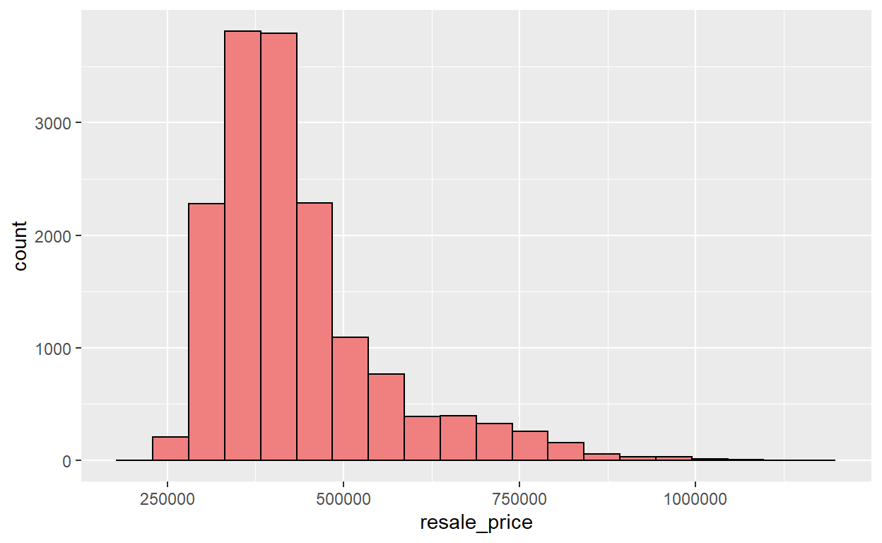
Results above reveals:

• A right skewed distribution.
• This means that more resale HDB units were transacted at relative lower prices.
  • Majority of the four room HDB units were transacted for about $300,000 to $450,000.
• Statistically, the skewed distribution can be normalised by using log transformation which we will be doing in the next section.

8.1.2 Normalise using Log Transformation

Here, we will:

• Derive a new variable called LOG_RESALE_PRICE by using a log transformation on the variable resale_price
• It is performed using mutate() of dplyr package.

rs_req <- rs_req %>%
  mutate(`LOG_SELLING_PRICE` = log(resale_price))

8.1.2 Plot Histogram of LOG_RESALE_PRICE

ggplot(data=rs_req, aes(x=`LOG_SELLING_PRICE`)) +
  geom_histogram(bins=20, color="black", fill="light green")

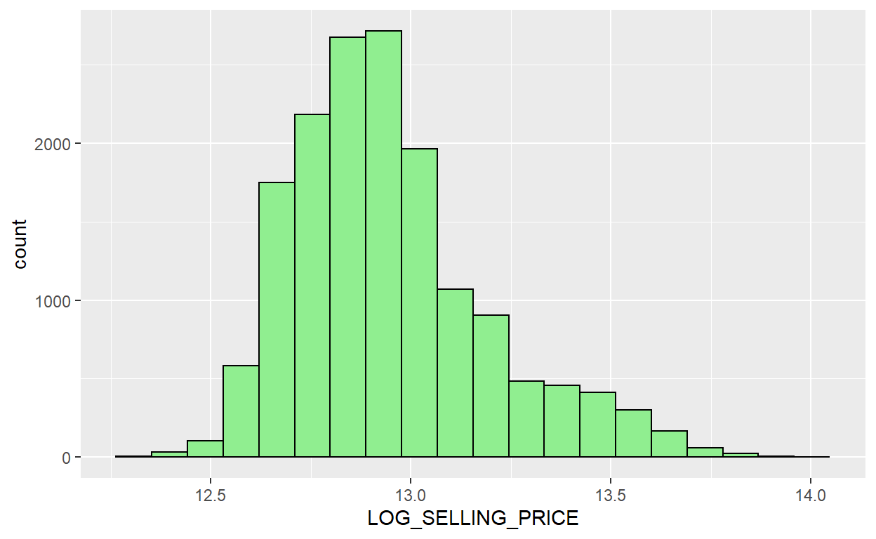
• The distribution is now relatively less skewed after the transformation.
• However, we will not be using this log resale price in our model as it will have a high correlation with our actual resale price.

8.2 Multiple Histogram Plots distribution of variables

8.2.1 Stuctural Factors

8.2.1.1 Extract column names to plot

s_factor <- c("floor_area_sqm", "storey_order", "remaining_lease_mths")

8.2.1.2 Create a list to store histograms of Stuctural Factors

• The following code chunk performs 3 steps:
  • 1. Creating a vector of the size of our structural factors called s_factor_hist_list
  • 2. Plotting a histogram for each of the structural factors
  • 3. Appending the histogram to the created vector

s_factor_hist_list <- vector(mode = "list", length = length(s_factor))
for (i in 1:length(s_factor)) {
  hist_plot <- ggplot(rs_req, aes_string(x = s_factor[[i]])) +
    geom_histogram(color="firebrick", fill = "light coral") +
    labs(title = s_factor[[i]]) +
    theme(plot.title = element_text(size = 10),
          axis.title = element_blank())
  
  s_factor_hist_list[[i]] <- hist_plot
}

8.2.1.3 Plot histograms to examine distribution of Stuctural Factors

Here we use ggarrange() function of ggpubr package to organise these histogram into a 2 columns by 2 rows small multiple plot.

ggarrange(plotlist = s_factor_hist_list,
          ncol = 2,
          nrow = 2)

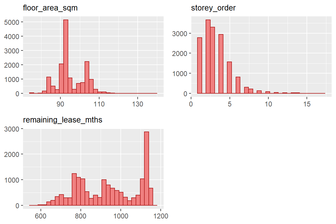
• From the results above, we can see that:
  • Only floor_area_sqm somewhat resembles a normal distribution.
  • Only storey_order has an obvious a right skew.
    • This means that the resale HDBs in this period and flat_type are generally on the lower levels.
  • remaining_lease_mths has 3 peaks found.
    • One near the 750 months, 900 months and 1100 months.
    • This can mean that there are generally 3 clusters of resale HDBs that are transacted with 62 years, 75 years and 91 years remaining, with the 3rd cluster having the highest number of resale HDBs.

8.2.2 Locational Factors

8.2.2.1 Extract column names to plot

• Note: Although there are discrete data in our locational factors like Within_threshold distance and more appropriate functions like geom_bar() or discrete.histogram() are recommended for this, we will still just plot a histogram as we are more interested in the distribution of the data.

l_factor <- c("PROX_CBD", "PROX_ELDERLYCARE", "PROX_HAWKER", "PROX_MRT", "PROX_PARK", "PROX_GOOD_PRISCH", "PROX_MALL", "PROX_CHAS",
              "PROX_SUPERMARKET", "WITHIN_350M_KINDERGARTEN", "WITHIN_350M_CHILDCARE", "WITHIN_350M_BUS", "WITHIN_1KM_PRISCH")

8.2.2.2 Create a list to store histograms of Locational Factors

• The following code chunk performs 3 steps:
  • 1. Creating a vector of the size of our locational factors called l_factor_hist_list
  • 2. Plotting a histogram for each of the locational factors
  • 3. Appending the histogram to the created vector

l_factor_hist_list <- vector(mode = "list", length = length(l_factor))
for (i in 1:length(l_factor)) {
  hist_plot <- ggplot(rs_req, aes_string(x = l_factor[[i]])) +
    geom_histogram(color="midnight blue", fill = "light sky blue") +
    labs(title = l_factor[[i]]) +
    theme(plot.title = element_text(size = 10),
          axis.title = element_blank())
  
  l_factor_hist_list[[i]] <- hist_plot
}

8.2.2.3 Plot histograms to examine distribution of Locational Factors

Here we use ggarrange() function of ggpubr package to organise these histogram into a 2 columns by 2 rows small multiple plot.

ggarrange(plotlist = l_factor_hist_list,
          ncol = 4,
          nrow = 4)

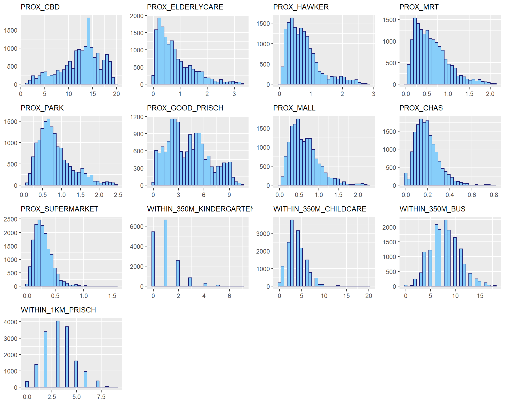
• From the results above, we can see that:
  • Only PROX_CBD have a somewhat left skewed distribution.
  • Only PROX_GOOD_PRISCH have 3 peaks found.
    • This can mean that there are generally 3 clusters of resale HDBs that are transacted with a proximity of about 2.8 km, 5.7km and 8.5km of good primary schools with more resale HDBs transacted with a proximity of about 2.8 km of good primary schools.
  • WITHIN_350M_BUS and WITHIN_1KM_PRISCH have a normal distribution.
  • Other variables like PROX_ELDERLYCARE, PROX_HAWKER, PROX_MRT, PROX_PARK, PROX_MALL, PROX_CHAS, PROX_SUPERMARKET, WITHIN_350M_KINDERGARTEN, WITHIN_350M_CHILDCARE have a right skewed distribution.

8.3 Statistical Point Map

tmap_mode("view")
tm_shape(rs_sf) +  
  tm_dots(col = "resale_price",
          alpha = 0.6,
          style="quantile") +
  tm_view(set.zoom.limits = c(11,14)) +
tm_basemap("OpenStreetMap")

tmap_mode("plot")

From the interactive map, we can see that 4 room HDBs in the Central and Northeast region tend to have higher resale prices which is indicated by the darker orange points. This is in comparison to the lighter yellow points concentrated around the North and West area.

9. Hedonic Pricing Modelling in R

• In this section, we will be performing regression analysis. Regression analysis is a set of statistical processes for explaining the relationships among variables. The focus is on the relationship between a dependent variable (y) and one or more independent variables (x).
• In this case, our y variable is HDB resale price while the x variables are the structural and locational factors. We are also particularly interested in finding out what is the change in price given a one unit change in the factors.
• We will also be performing both Simple and Multiple Linear Regression (MLR) Analysis to get a sense of what is the difference between the 2 instead of jumping straight to MLR.

9.1 Simple Linear Regression (SLR) Model

9.1.1 Combine structural and locational factors list

factors <- c(s_factor, l_factor)
factors

 [1] "floor_area_sqm"           "storey_order"            
 [3] "remaining_lease_mths"     "PROX_CBD"                
 [5] "PROX_ELDERLYCARE"         "PROX_HAWKER"             
 [7] "PROX_MRT"                 "PROX_PARK"               
 [9] "PROX_GOOD_PRISCH"         "PROX_MALL"               
[11] "PROX_CHAS"                "PROX_SUPERMARKET"        
[13] "WITHIN_350M_KINDERGARTEN" "WITHIN_350M_CHILDCARE"   
[15] "WITHIN_350M_BUS"          "WITHIN_1KM_PRISCH"       

9.1.2 Build Simple Linear Regression model

• Here we will,
  • Build multiple Simple Linear Regression models built using resale_price and factors like structural and locational.
  • The purpose of building these models is so that we can see for ourselves what is the linear relationship between resale_price and each of the factor.

Code Chunk

intercept_df <- data.frame()
rsq_fstat_df <- data.frame()

for (i in factors){
  rs_slr <- lm(as.formula(paste("resale_price", "~", i)), data = rs_req)
  intercept <- tidy(summary(rs_slr))
  intercept$var_name <- i
  rsq_fstat <- glance(rs_slr)[1:5]
  rsq_fstat$var_name <- i
  # Append
  intercept_df <- bind_rows(intercept_df, intercept)
  rsq_fstat_df <- bind_rows(rsq_fstat_df, rsq_fstat)
}

Intercept

intercept_df

                       term     estimate    std.error    statistic
1               (Intercept)  527814.1890 12779.676387   41.3010606
2            floor_area_sqm    -990.2711   133.936427   -7.3935909
3               (Intercept)  335918.3804  1614.399924  208.0763108
4              storey_order   29974.1751   424.719502   70.5740493
5               (Intercept)  174540.0791  5505.512832   31.7027831
6      remaining_lease_mths     275.6416     5.780934   47.6811567
7               (Intercept)  663301.8862  2351.552372  282.0697910
8                  PROX_CBD  -18323.1853   178.093597 -102.8851439
9               (Intercept)  474058.4891  1444.405678  328.2031470
10         PROX_ELDERLYCARE  -50059.3753  1381.858792  -36.2261149
11              (Intercept)  483151.1427  1635.303435  295.4504543
12              PROX_HAWKER  -64847.4551  1773.410597  -36.5665206
13              (Intercept)  477708.8356  1728.655991  276.3469644
14                 PROX_MRT  -72349.1554  2393.285050  -30.2300620
15              (Intercept)  478426.1153  1955.487499  244.6582325
16                PROX_PARK  -54229.6508  2078.633240  -26.0890905
17              (Intercept)  503380.8355  1775.259885  283.5533207
18         PROX_GOOD_PRISCH  -16666.5666   365.981906  -45.5393185
19              (Intercept)  436784.2505  1942.247089  224.8860369
20                PROX_MALL   -5026.5299  2662.295137   -1.8880438
21              (Intercept)  472102.4744  1912.352836  246.8699632
22                PROX_CHAS -200045.5965  8658.881082  -23.1029384
23              (Intercept)  472048.5413  1929.847287  244.6040909
24         PROX_SUPERMARKET -135816.1182  5956.970219  -22.7995295
25              (Intercept)  433191.0027  1348.649690  321.2035014
26 WITHIN_350M_KINDERGARTEN     393.0328   944.040535    0.4163305
27              (Intercept)  444654.4226  2099.881066  211.7521939
28    WITHIN_350M_CHILDCARE   -2852.7865   482.573065   -5.9116157
29              (Intercept)  459759.3601  2772.086222  165.8531962
30          WITHIN_350M_BUS   -3278.6824   326.273978  -10.0488627
31              (Intercept)  494036.8907  2186.039156  225.9963594
32        WITHIN_1KM_PRISCH  -18450.7246   604.444230  -30.5251066
         p.value                 var_name
1   0.000000e+00           floor_area_sqm
2   1.500304e-13           floor_area_sqm
3   0.000000e+00             storey_order
4   0.000000e+00             storey_order
5  6.124051e-214     remaining_lease_mths
6   0.000000e+00     remaining_lease_mths
7   0.000000e+00                 PROX_CBD
8   0.000000e+00                 PROX_CBD
9   0.000000e+00         PROX_ELDERLYCARE
10 3.483362e-276         PROX_ELDERLYCARE
11  0.000000e+00              PROX_HAWKER
12 3.727348e-281              PROX_HAWKER
13  0.000000e+00                 PROX_MRT
14 3.056832e-195                 PROX_MRT
15  0.000000e+00                PROX_PARK
16 5.900357e-147                PROX_PARK
17  0.000000e+00         PROX_GOOD_PRISCH
18  0.000000e+00         PROX_GOOD_PRISCH
19  0.000000e+00                PROX_MALL
20  5.903826e-02                PROX_MALL
21  0.000000e+00                PROX_CHAS
22 3.517208e-116                PROX_CHAS
23  0.000000e+00         PROX_SUPERMARKET
24 3.013018e-113         PROX_SUPERMARKET
25  0.000000e+00 WITHIN_350M_KINDERGARTEN
26  6.771738e-01 WITHIN_350M_KINDERGARTEN
27  0.000000e+00    WITHIN_350M_CHILDCARE
28  3.457020e-09    WITHIN_350M_CHILDCARE
29  0.000000e+00          WITHIN_350M_BUS
30  1.093661e-23          WITHIN_350M_BUS
31  0.000000e+00        WITHIN_1KM_PRISCH
32 6.343926e-199        WITHIN_1KM_PRISCH

R-square

rsq_fstat_df

      r.squared adj.r.squared     sigma    statistic       p.value
1  3.426497e-03  3.363816e-03 119917.98 5.466519e+01  1.500304e-13
2  2.385426e-01  2.384947e-01 104822.00 4.980696e+03  0.000000e+00
3  1.251063e-01  1.250512e-01 112358.85 2.273493e+03  0.000000e+00
4  3.996833e-01  3.996455e-01  93072.18 1.058535e+04  0.000000e+00
5  7.624810e-02  7.619000e-02 115453.56 1.312331e+03 3.483362e-276
6  7.757611e-02  7.751809e-02 115370.54 1.337110e+03 3.727348e-281
7  5.435463e-02  5.429515e-02 116813.70 9.138566e+02 3.056832e-195
8  4.105280e-02  4.099248e-02 117632.41 6.806406e+02 5.900357e-147
9  1.153869e-01  1.153313e-01 112981.24 2.073830e+03  0.000000e+00
10 2.241594e-04  1.612765e-04 120110.50 3.564710e+00  5.903826e-02
11 3.248062e-02  3.241977e-02 118157.01 5.337458e+02 3.517208e-116
12 3.165992e-02  3.159902e-02 118207.11 5.198185e+02 3.013018e-113
13 1.090189e-05 -5.199446e-05 120123.31 1.733311e-01  6.771738e-01
14 2.193254e-03  2.130495e-03 119992.16 3.494720e+01  3.457020e-09
15 6.311236e-03  6.248735e-03 119744.30 1.009796e+02  1.093661e-23
16 5.536178e-02  5.530237e-02 116751.48 9.317821e+02 6.343926e-199
                   var_name
1            floor_area_sqm
2              storey_order
3      remaining_lease_mths
4                  PROX_CBD
5          PROX_ELDERLYCARE
6               PROX_HAWKER
7                  PROX_MRT
8                 PROX_PARK
9          PROX_GOOD_PRISCH
10                PROX_MALL
11                PROX_CHAS
12         PROX_SUPERMARKET
13 WITHIN_350M_KINDERGARTEN
14    WITHIN_350M_CHILDCARE
15          WITHIN_350M_BUS
16        WITHIN_1KM_PRISCH

From the results above, we can see that:

• The resale_price can be explained by using many different formulas. For example, looking at the estimates at Intercept and storey_order, the formula can be defined as:

\[ y = 335918.3804 + 29974.1751 x1 \]

• The model with the highest Multiple R-squared value is the Simple Linear Regression Model of resale_price and PROX_HAWKER with a value of 7.757611e-02 or 0.07757611 of while the model with the lowest Multiple R-squared value is the Simple Linear Regression Model of resale_price and WITHIN_350M_KINDERGARTEN with a value of 1.090189e-05 or 0.00001090189.
  • This means that the Simple Linear Regression Model with PROX_HAWKER as the independent variable is able to explain about 7% of the resale price which is quite low however still higher than the Simple Linear Regression Model with WITHIN_350M_KINDERGARTEN as the independent variable as the lowest Multiple R-squared value of much less than 0.00001.
• Since our p-value of all the Simple Linear Regression models are much smaller than 0.0001, we will reject the null hypothesis that the mean is a good estimator of resale_price and we can infer that the Simple Linear Regression model above is a good estimator of resale_price.
• The coefficients reveals that the p-values of both the estimates of the Intercepts and all of the factors are smaller than 0.001.
  • Within this context, the null hypothesis of the B0 and B1 are equal to 0 will be rejected.
  • As such, we can infer that B0 and B1 are good parameter estimates.

9.1.3 Visualise best fit curve

• To visualise the best fit curve on a scatterplot, we can incorporate lm() as a method function in ggplot’s geometry as shown in the code chunk below.
• In this analysis, I have also changed the parameter of aes() to aes_string() since we want to automate the plotting of multiple best fit curve of the Simple Linear Regression models.

scatterplot_list <- vector(mode = "list", length = length(factors))

for (i in factors){
  scatterplot <- ggplot(data=rs_req,
                        aes_string(x=i, y="resale_price")) + 
    geom_point() + geom_smooth(method = lm)
  scatterplot_list[[i]] <- scatterplot
}

ggarrange(plotlist = scatterplot_list, ncol = 4, nrow = 4)

$`1`

$`2`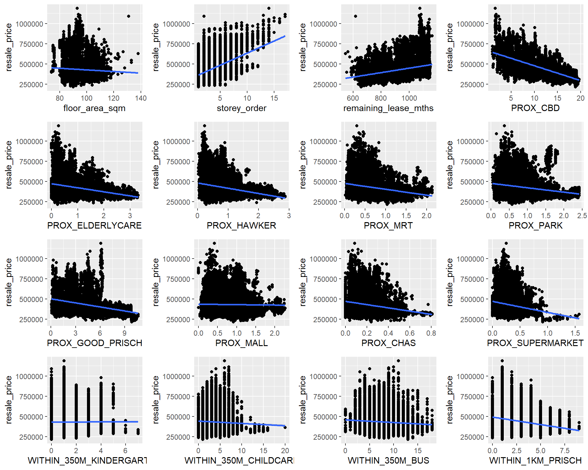

attr(,"class")
[1] "list"      "ggarrange"

From the results above, we can see that:

• There is some relationship between the resale_price and independent variables. We can also see an upward slope and downward slope with a straight-line pattern in the plotted data points.
  • For example, value for resale_price does tend to decrease as the PROX_CBD decreases
  • Similarly, value for resale_price does tend to increase as the remaining_lease_mths increases
  • A strong relationship between the dependent variable and the independent variable tend to lead to a good model
• There are also a few statistical outliers with relatively high selling prices.

Overall,

• Although there are some indications that these variables can help to explain and predict the resale price, we must still remember that the adjusted R squared value that we saw earlier on is quite low which means it is able to explain only a small percentage of the resale prices.
• Since there are multiple variables that we can use, we can now try to build Multiple Linear Regression Model to see if there is a huge difference.

9.2 Multiple Linear Regression Model

• Multiple linear regression allows us to account for all of these potentially important factors in one model.
  • The advantages of this approach are that this may lead to a more accurate and precise understanding of the association of each individual factor with the outcome.
• However, before we proceed, we need to know whether there are any redundant independent variables.
• As such, we need to ensure that the independent variables used are not highly correlated to each other.
  • If these highly correlated independent variables are used in building a regression model, the quality of the model will be compromised.
  • This phenomena is known as multicollinearity in statistics.
• Correlation matrix is commonly used to visualise the relationships between the independent variables.

9.2.1 Visualise relationships of independent variables

9.2.1.1 Set geometry as null first

Code Chunk

rs_req_nogeom <- st_set_geometry(rs_req, NULL) 

Glimpse

glimpse(rs_req_nogeom)

Rows: 15,901
Columns: 18
$ resale_price             <dbl> 330000, 360000, 370000, 375000, 380~
$ floor_area_sqm           <dbl> 92, 91, 92, 99, 92, 92, 92, 92, 93,~
$ storey_order             <int> 1, 3, 1, 2, 2, 4, 3, 2, 4, 3, 3, 3,~
$ remaining_lease_mths     <dbl> 684, 738, 733, 700, 715, 732, 706, ~
$ PROX_CBD                 <dbl> 8.824749, 9.841309, 9.560780, 9.609~
$ PROX_ELDERLYCARE         <dbl> 0.2514065, 0.6318448, 1.0824168, 0.~
$ PROX_HAWKER              <dbl> 0.44182653, 0.26972560, 0.25829513,~
$ PROX_MRT                 <dbl> 0.6885144, 1.0969096, 0.8862859, 1.~
$ PROX_PARK                <dbl> 0.7450859, 0.4294870, 0.7800777, 0.~
$ PROX_GOOD_PRISCH         <dbl> 1.2703931, 0.4045792, 2.0942375, 0.~
$ PROX_MALL                <dbl> 0.5534331, 1.0677012, 0.9751113, 1.~
$ PROX_CHAS                <dbl> 1.364596e-01, 2.569863e-01, 1.90618~
$ PROX_SUPERMARKET         <dbl> 0.2708222, 0.3101889, 0.3187560, 0.~
$ WITHIN_350M_KINDERGARTEN <int> 1, 1, 1, 1, 1, 1, 1, 1, 1, 0, 1, 1,~
$ WITHIN_350M_CHILDCARE    <int> 6, 5, 2, 3, 3, 2, 3, 4, 3, 2, 4, 4,~
$ WITHIN_350M_BUS          <int> 8, 8, 8, 7, 6, 9, 6, 6, 5, 4, 10, 5~
$ WITHIN_1KM_PRISCH        <int> 2, 2, 1, 2, 2, 1, 3, 2, 2, 2, 2, 2,~
$ LOG_SELLING_PRICE        <dbl> 12.70685, 12.79386, 12.82126, 12.83~

9.2.1.2 Plot a scatterplot matrix

• Here we use corrplot() function of corrplot package to visualise the relationships between the independent variables.
• tl.cex is set to 0.8 so that the variables are more visible.

corrplot(cor(rs_req_nogeom[, 2:17]), diag = FALSE, order = "AOE",
          tl.pos = "td", tl.cex = 0.8, method = "number", type = "upper")

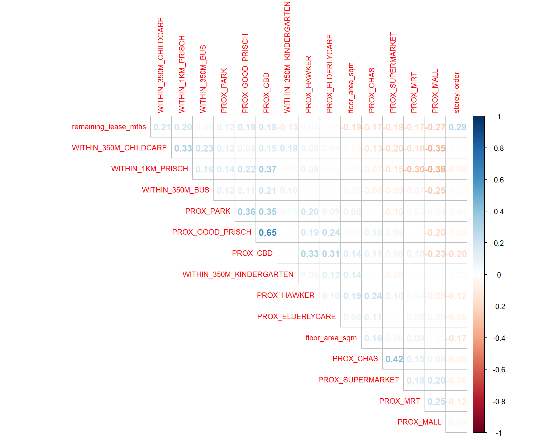
• From the scatterplot matrix, it is clear that PROX_GOOD_PRISCH is moderately correlated to PROX_CBD.
• In view of this, it is wiser to only include either one of them in the subsequent model building.
  • You can try to include it in the model and see what adjusted r square value you get at the end of this analysis! :)
  • PS, I did try including the variable PROX_GOOD_PRISCH considering how both variables are not highly correlated as I thought they were. However, the final adjusted r square value that I obtained at the end of this exercise was lower than the model with the excluded PROX_GOOD_PRISCH.
• As a result, PROX_GOOD_PRISCH will be excluded in the subsequent model building.

9.2.2 Hedonic Pricing Model Using Multiple Linear Regression Method

9.2.2.1 Calibrate The Multiple Linear Regression Model

• Here we use lm() function of stats package to calibrate the multiple linear regression model.
• Note: PROX_GOOD_PRISCH is excluded in this model.

rs_mlr1 <- lm(formula = resale_price ~ floor_area_sqm + storey_order + remaining_lease_mths + PROX_CBD + PROX_ELDERLYCARE + PROX_HAWKER + PROX_MRT + PROX_PARK + PROX_MALL +  PROX_CHAS + PROX_SUPERMARKET + WITHIN_350M_KINDERGARTEN + WITHIN_350M_CHILDCARE + WITHIN_350M_BUS + WITHIN_1KM_PRISCH, data=rs_req)
summary(rs_mlr1)

Call:
lm(formula = resale_price ~ floor_area_sqm + storey_order + remaining_lease_mths + 
    PROX_CBD + PROX_ELDERLYCARE + PROX_HAWKER + PROX_MRT + PROX_PARK + 
    PROX_MALL + PROX_CHAS + PROX_SUPERMARKET + WITHIN_350M_KINDERGARTEN + 
    WITHIN_350M_CHILDCARE + WITHIN_350M_BUS + WITHIN_1KM_PRISCH, 
    data = rs_req)

Residuals:
    Min      1Q  Median      3Q     Max 
-205053  -39222   -1322   36087  470016 

Coefficients:
                           Estimate Std. Error  t value Pr(>|t|)    
(Intercept)              111623.296   8620.295   12.949  < 2e-16 ***
floor_area_sqm             2772.976     73.210   37.877  < 2e-16 ***
storey_order              14176.792    273.075   51.915  < 2e-16 ***
remaining_lease_mths        343.444      3.717   92.393  < 2e-16 ***
PROX_CBD                 -17081.837    162.184 -105.324  < 2e-16 ***
PROX_ELDERLYCARE         -13822.538    801.751  -17.240  < 2e-16 ***
PROX_HAWKER              -19378.130   1047.804  -18.494  < 2e-16 ***
PROX_MRT                 -33416.893   1405.382  -23.778  < 2e-16 ***
PROX_PARK                 -5303.822   1191.761   -4.450 8.63e-06 ***
PROX_MALL                -15888.940   1626.410   -9.769  < 2e-16 ***
PROX_CHAS                 -3552.549   5190.994   -0.684    0.494    
PROX_SUPERMARKET         -24869.905   3599.407   -6.909 5.05e-12 ***
WITHIN_350M_KINDERGARTEN   7971.900    510.602   15.613  < 2e-16 ***
WITHIN_350M_CHILDCARE     -4228.627    285.192  -14.827  < 2e-16 ***
WITHIN_350M_BUS             952.733    179.548    5.306 1.13e-07 ***
WITHIN_1KM_PRISCH         -8359.331    393.880  -21.223  < 2e-16 ***
---
Signif. codes:  0 '***' 0.001 '**' 0.01 '*' 0.05 '.' 0.1 ' ' 1

Residual standard error: 61410 on 15885 degrees of freedom
Multiple R-squared:  0.7389,    Adjusted R-squared:  0.7386 
F-statistic:  2997 on 15 and 15885 DF,  p-value: < 2.2e-16

Results above show that:

• Only the PROX_CHAS independent variable is not statistically significant.
• We will revise the model by removing this variable which is not statistically significant.
• Also, by adding more variables, the adjusted r square actually improved drastically from the previous 0.07757611 to about 0.7389. Yay! :D
• This now means that the remaining independent variables here are able to explain about 74% of the resale prices!

9.2.2.1 Calibrate The Revised Multiple Linear Regression Model

• Now, we are ready to calibrate the revised model by using the code chunk below.
• Ordinary least squares regression is then performed using ols_regress() function of olsrr package.

rs_mlr1 <- lm(formula = resale_price ~ floor_area_sqm + storey_order + remaining_lease_mths + PROX_CBD + PROX_ELDERLYCARE + PROX_HAWKER + PROX_MRT + PROX_PARK + PROX_MALL  + PROX_SUPERMARKET + WITHIN_350M_KINDERGARTEN + WITHIN_350M_CHILDCARE + WITHIN_350M_BUS + WITHIN_1KM_PRISCH, data=rs_req)
ols_regress(rs_mlr1)

                            Model Summary                              
----------------------------------------------------------------------
R                       0.860       RMSE                    61410.034 
R-Squared               0.739       Coef. Var                  14.163 
Adj. R-Squared          0.739       MSE                3771192239.771 
Pred R-Squared          0.738       MAE                     47325.690 
----------------------------------------------------------------------
 RMSE: Root Mean Square Error 
 MSE: Mean Square Error 
 MAE: Mean Absolute Error 

                                     ANOVA                                       
--------------------------------------------------------------------------------
                    Sum of                                                      
                   Squares           DF       Mean Square       F          Sig. 
--------------------------------------------------------------------------------
Regression    1.695097e+14           14      1.210783e+13    3210.612    0.0000 
Residual      5.990916e+13        15886    3771192239.771                       
Total         2.294188e+14        15900                                         
--------------------------------------------------------------------------------

                                                Parameter Estimates                                                 
-------------------------------------------------------------------------------------------------------------------
                   model          Beta    Std. Error    Std. Beta       t         Sig          lower         upper 
-------------------------------------------------------------------------------------------------------------------
             (Intercept)    111463.459      8616.986                   12.935    0.000     94573.189    128353.728 
          floor_area_sqm      2768.830        72.957        0.164      37.951    0.000      2625.826      2911.834 
            storey_order     14173.718       273.034        0.231      51.912    0.000     13638.540     14708.895 
    remaining_lease_mths       343.671         3.702        0.441      92.825    0.000       336.414       350.928 
                PROX_CBD    -17080.790       162.174       -0.589    -105.324    0.000    -17398.670    -16762.911 
        PROX_ELDERLYCARE    -13875.497       797.994       -0.077     -17.388    0.000    -15439.656    -12311.339 
             PROX_HAWKER    -19510.231      1029.854       -0.084     -18.945    0.000    -21528.861    -17491.601 
                PROX_MRT    -33473.302      1402.939       -0.108     -23.859    0.000    -36223.222    -30723.383 
               PROX_PARK     -5324.828      1191.346       -0.020      -4.470    0.000     -7660.001     -2989.655 
               PROX_MALL    -15836.175      1624.554       -0.047      -9.748    0.000    -19020.485    -12651.864 
        PROX_SUPERMARKET    -25785.939      3341.220       -0.034      -7.718    0.000    -32335.108    -19236.770 
WITHIN_350M_KINDERGARTEN      7975.889       510.561        0.067      15.622    0.000      6975.133      8976.646 
   WITHIN_350M_CHILDCARE     -4220.040       284.911       -0.069     -14.812    0.000     -4778.497     -3661.583 
         WITHIN_350M_BUS       958.788       179.327        0.023       5.347    0.000       607.287      1310.289 
       WITHIN_1KM_PRISCH     -8362.395       393.848       -0.107     -21.233    0.000     -9134.381     -7590.408 
-------------------------------------------------------------------------------------------------------------------

• Here our rs_mlr1 will contain the coefficients, residuals, effects and fitted values.
• We will be using the residuals and extract it as a dataframe later on to examine it closely.

9.2.3 Check for multicolinearity

• Here, ols_vif_tol() function of olsrr package is used to check if there are any strong signs of multicollinearity.

ols_vif_tol(rs_mlr1)

                  Variables Tolerance      VIF
1            floor_area_sqm 0.8838343 1.131434
2              storey_order 0.8305099 1.204080
3      remaining_lease_mths 0.7282816 1.373095
4                  PROX_CBD 0.5250169 1.904701
5          PROX_ELDERLYCARE 0.8483834 1.178712
6               PROX_HAWKER 0.8401490 1.190265
7                  PROX_MRT 0.8042711 1.243362
8                 PROX_PARK 0.8296684 1.205301
9                 PROX_MALL 0.7020382 1.424424
10         PROX_SUPERMARKET 0.8578914 1.165649
11 WITHIN_350M_KINDERGARTEN 0.8935338 1.119152
12    WITHIN_350M_CHILDCARE 0.7514186 1.330816
13          WITHIN_350M_BUS 0.8706491 1.148568
14        WITHIN_1KM_PRISCH 0.6516424 1.534584

Since all the VIF values of the independent variables are less than 10, we can safely conclude that there is no signs of multicollinearity among the independent variables.

9.2.4 Test for Non-Linearity

ols_plot_resid_fit(rs_mlr1)

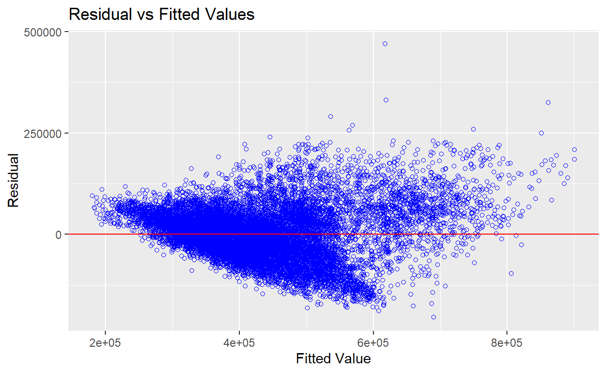
Results above show that:

• Most of the data points are scattered around the 0 line.
• Hence, we can safely conclude that the relationships between the dependent variable and independent variables are linear.

9.2.5 Test for Normality Assumption

• For formal statistical test methods, the ols_test_normality() of olsrr package can be used as well.
• However, since our sample size is more than 5000, we will not be using this function for this analysis.
• Instead, we will be using ols_plot_resid_hist() of olsrr package to perform normality assumption test.

ols_plot_resid_hist(rs_mlr1)

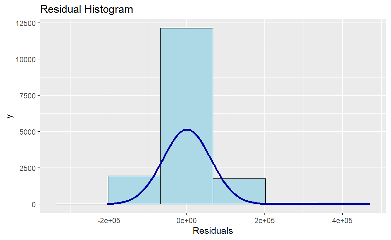
Results above reveals that the residual of the multiple linear regression model (i.e. rs_mlr1) resembles a normal distribution.

9.2.6 Test for Spatial Autocorrelation

• The hedonic model we try to build are using geographically referenced attributes.
• Hence it is also important for us to visualse the residual of the hedonic pricing model.
• In order to perform spatial autocorrelation test, we need to convert rs_req into a SpatialPointsDataFrame.
• First, we will export the residual of the hedonic pricing model and save it as a data frame.
• Next, we will join the newly created data frame with rs_req object.
• Then, we will convert rs.res.sf simple feature object into a SpatialPointsDataFrame because spdep package can only process sp conformed spatial data objects

9.2.6.1 Export residual of hedonic pricing model

mlr.output <- as.data.frame(rs_mlr1$residuals)

9.2.6.2 Join with condo_resale.sf object

Code Chunk

rs.res.sf <- cbind(rs_req,
                   rs_mlr1$residuals) %>%
rename(`MLR_RES` = `rs_mlr1.residuals`)

Glimpse

glimpse(rs.res.sf)

Rows: 15,901
Columns: 20
$ resale_price             <dbl> 330000, 360000, 370000, 375000, 380~
$ floor_area_sqm           <dbl> 92, 91, 92, 99, 92, 92, 92, 92, 93,~
$ storey_order             <int> 1, 3, 1, 2, 2, 4, 3, 2, 4, 3, 3, 3,~
$ remaining_lease_mths     <dbl> 684, 738, 733, 700, 715, 732, 706, ~
$ PROX_CBD                 <dbl> 8.824749, 9.841309, 9.560780, 9.609~
$ PROX_ELDERLYCARE         <dbl> 0.2514065, 0.6318448, 1.0824168, 0.~
$ PROX_HAWKER              <dbl> 0.44182653, 0.26972560, 0.25829513,~
$ PROX_MRT                 <dbl> 0.6885144, 1.0969096, 0.8862859, 1.~
$ PROX_PARK                <dbl> 0.7450859, 0.4294870, 0.7800777, 0.~
$ PROX_GOOD_PRISCH         <dbl> 1.2703931, 0.4045792, 2.0942375, 0.~
$ PROX_MALL                <dbl> 0.5534331, 1.0677012, 0.9751113, 1.~
$ PROX_CHAS                <dbl> 1.364596e-01, 2.569863e-01, 1.90618~
$ PROX_SUPERMARKET         <dbl> 0.2708222, 0.3101889, 0.3187560, 0.~
$ WITHIN_350M_KINDERGARTEN <int> 1, 1, 1, 1, 1, 1, 1, 1, 1, 0, 1, 1,~
$ WITHIN_350M_CHILDCARE    <int> 6, 5, 2, 3, 3, 2, 3, 4, 3, 2, 4, 4,~
$ WITHIN_350M_BUS          <int> 8, 8, 8, 7, 6, 9, 6, 6, 5, 4, 10, 5~
$ WITHIN_1KM_PRISCH        <int> 2, 2, 1, 2, 2, 1, 3, 2, 2, 2, 2, 2,~
$ LOG_SELLING_PRICE        <dbl> 12.70685, 12.79386, 12.82126, 12.83~
$ MLR_RES                  <dbl> -53437.543, -31360.769, -20277.877,~
$ geometry                 <POINT [m]> POINT (29179.92 38822.08), PO~

9.2.6.3 Convert to spatialpointsdataframe

rs.sp <- as_Spatial(rs.res.sf)
rs.sp

class       : SpatialPointsDataFrame 
features    : 15901 
extent      : 11597.31, 42623.63, 28217.39, 48741.06  (xmin, xmax, ymin, ymax)
crs         : +proj=tmerc +lat_0=1.36666666666667 +lon_0=103.833333333333 +k=1 +x_0=28001.642 +y_0=38744.572 +ellps=WGS84 +towgs84=0,0,0,0,0,0,0 +units=m +no_defs 
variables   : 19
names       : resale_price, floor_area_sqm, storey_order, remaining_lease_mths,          PROX_CBD,     PROX_ELDERLYCARE,        PROX_HAWKER,           PROX_MRT,          PROX_PARK,   PROX_GOOD_PRISCH,        PROX_MALL,            PROX_CHAS,     PROX_SUPERMARKET, WITHIN_350M_KINDERGARTEN, WITHIN_350M_CHILDCARE, ... 
min values  :       218000,             74,            1,                  546, 0.999393538715878, 1.98943787433087e-08, 0.0333358643817954, 0.0220407324774434, 0.0441643212802781, 0.0652540365486641,                0, 4.55547870890763e-09, 1.21715176356525e-07,                        0,                     0, ... 
max values  :      1186888,            138,           17,                 1164,  19.6500691667807,     3.30163731686804,   2.86763031236184,   2.13060636038504,   2.41313695915468,   10.6223726149914, 2.27100643784442,    0.808332738794272,     1.57131703651196,                        7,                    20, ... 

9.2.6.4 Display interactive point symbol map

• Next, we will use tmap package to display the distribution of the residuals.

tmap_mode("view")
tm_basemap("OpenStreetMap")+
tm_shape(mpsz_sf)+
  tm_polygons(alpha = 0.4) +
tm_shape(rs.res.sf) +  
  tm_dots(col = "MLR_RES",
          alpha = 0.6,
          style="quantile") +
  tm_view(set.zoom.limits = c(11,14))

tmap_mode("plot")

• From the plot above, we can see that there is somewhat spatial autocorrelation where similar values tend to be in similar location.
• However, to confirm that there truly is spatial autocorrelation, we will perform Moran’s I test to validate our claims.

9.3 Moran’s I test

9.3.1 Obtaining upper distance band

coords <- coordinates(rs.sp)
k <- knn2nb(knearneigh(coords))
kdists <- unlist(nbdists(k, coords, longlat=FALSE))
summary(kdists)

    Min.  1st Qu.   Median     Mean  3rd Qu.     Max. 
   0.000    0.000    0.000    6.771    0.000 1485.733 

Looking at the output we would be using 1500 as the max band.

9.3.2 Compute the distance-based weight matrix

• Compute the distance-based weight matrix by using dnearneigh() of spdep package

nb <- dnearneigh(coordinates(rs.sp), 0, 1500, longlat = FALSE)
summary(nb)

Neighbour list object:
Number of regions: 15901 
Number of nonzero links: 10219568 
Percentage nonzero weights: 4.041882 
Average number of links: 642.6997 
Link number distribution:

   2    7   14   25   26   31   32   46   56   57   60   65   68   69 
   3    1   14   15    5    4    2   47    4    4    5    2    4    1 
  71   72   75   79   86   88   89   90   97   99  101  103  106  109 
  12    1    1   78    3    5    4    3    8    8    6    2    2    5 
 110  112  115  117  118  119  120  121  122  123  124  125  126  128 
   8    3    6    1    9    6    5    7    4   22    7   55   21   30 
 130  131  132  133  134  135  136  137  138  139  140  141  142  143 
   1   14    6   14    7    5    5    9    2   28    4    2    8   15 
 145  146  147  148  149  150  151  152  153  154  155  156  157  158 
   9    6   17    6    1    1   21   20   13    7    3    8    9    5 
 159  160  161  162  163  164  165  166  167  168  169  170  171  173 
  17    6    3    2   12    6    6    3   11    3   11    3    8   14 
 174  175  176  177  178  179  180  181  182  183  184  185  186  187 
   2   28   14   23   10   17   11    7    5   12   12    9   37   22 
 188  189  190  191  192  193  194  195  196  197  198  199  200  201 
  14    3    5    6   10    7    2    8    4    7   21    8   14   18 
 202  203  204  205  206  207  208  209  210  211  212  213  214  215 
  28    3   15   14    3    5   22    4    1    5    8    4   14   21 
 216  217  218  219  220  221  222  223  224  225  226  227  228  229 
   6    3    2   12   24   28   38    3   10   10    4   20   25    3 
 230  231  232  233  234  235  236  237  238  239  240  241  242  243 
  10   15    3   14   13   37   10    2   21   10   32   23    8    8 
 244  245  246  247  248  249  250  251  252  253  254  255  256  257 
  11   11    3   14   13   20    6   24    8   23   18   15   15   13 
 258  259  260  261  262  263  264  265  266  267  268  269  270  271 
   7    4    7   11   14    5   17   13    3   27   34   24    1   19 
 272  273  274  275  276  277  278  279  280  281  282  283  284  285 
  34   55   19   20   23   17   58   12   54   29   31   24   33   27 
 286  287  288  289  290  291  292  293  294  295  296  297  298  299 
  12   62   50   29   21   33   71   39   17   43    8   17   30   25 
 300  301  302  303  304  305  306  307  308  309  310  311  312  313 
  21   23   34   21   31   32   22   12   19    4   13   12   10   24 
 314  315  316  317  318  319  320  321  322  323  324  325  326  327 
   7   26   18   16   44   22   19   22   26   24   39   21   19   42 
 328  329  330  331  332  333  334  335  336  337  338  339  340  341 
  24   23   23   31   12   19   27   34    3   27   35   25   21   42 
 342  343  344  345  346  347  348  349  350  351  352  353  354  355 
   6   28   19   18   12   28   10   41   20   23   32   10   34   30 
 356  357  358  359  360  361  362  363  364  365  366  367  368  369 
  20    6   20   17   43   24    7   13   43   12   42   31   11   36 
 370  371  372  373  374  375  376  377  378  379  380  381  382  383 
   5   31   17   17   45   19   37   35   10   24   14   13   23   17 
 384  385  386  387  388  389  390  391  392  393  394  395  396  397 
   4   35   32   31   22   16   40   15   16   16   20   22   23   31 
 398  399  400  401  402  403  404  405  406  407  408  409  410  411 
  19   12   27   21   24   18   32    8   16   16   23    3   23   18 
 412  413  414  415  416  417  418  419  420  421  422  423  424  425 
  26   22    9   26   16   14   13   66   20   12   13   82   14   19 
 426  427  428  429  430  431  432  433  434  435  436  437  438  439 
  25   23   30   26    9   29   18   29   32   20   35   12   25   21 
 440  441  442  443  444  445  446  447  448  449  450  451  452  453 
  14   27   11   10    1   27   10   13   27   24   15   11   35   26 
 454  455  456  457  458  459  460  461  462  463  464  465  466  467 
  11   25   21   17   58   33    3   15   17    6   31   15    7   23 
 468  469  470  471  472  473  474  475  476  477  478  479  480  481 
  28    6   16   21    9   19   23    8   24   16   33   30   25   20 
 482  483  484  485  486  487  488  489  490  491  492  493  494  495 
  13    9    8   23   17   12   15   10   34    8    4   18   11   20 
 496  497  498  499  500  501  502  503  504  505  506  507  508  509 
   5   19    6    8   10    5    4   26   17   22   10   41   18    6 
 510  511  512  513  514  515  516  517  518  519  520  521  522  523 
  24   34   28   34    1   13   14    4    7    7    7    4    9   18 
 524  525  526  527  528  529  530  531  532  533  534  535  536  537 
  11   10    8   10    7   50   21   14   20   12   10   17   21    7 
 538  539  540  541  542  543  544  545  546  547  548  549  550  551 
   3    9    4    6    3   16   24   15   11    5    8   13    8   18 
 552  553  554  555  556  557  558  559  560  561  562  563  564  565 
   8    9    5   12    5   11   18   22   12    7    5   21   10   15 
 566  567  568  569  570  571  572  573  574  575  576  577  578  579 
  33   17   22   15   12   17    7    8   21   17   42    4   27    8 
 580  582  583  584  585  586  587  588  589  590  591  592  593  594 
  13   10   10   16    7   20   13    5   12   31   20   22    8   13 
 595  596  597  598  599  600  601  602  603  604  605  606  607  608 
  13   13   24   12    8   17   11    6   12   18   10    3   18   11 
 609  610  611  612  613  614  615  616  617  618  619  620  621  622 
  12   14   25   26    7    9   10    7   27   26   12    4   10    1 
 623  624  625  626  627  628  629  630  631  632  633  634  635  636 
   2   26    7   14   21   16    5    5    7    4    3   22    4   13 
 637  638  639  640  641  642  643  644  645  646  647  648  649  650 
  19   24    5    8    5   17    9    7   14    3   33   10    5   14 
 651  652  653  654  655  656  657  658  659  660  661  662  664  666 
   5   39    9    5   10   10    5    4    2   11   21    4   18    3 
 667  668  669  670  671  672  673  674  675  676  677  678  679  680 
   2    4   17   14   15    5    9    3    9   25    6    9   13   14 
 681  682  683  684  686  687  688  689  690  691  692  693  694  695 
   8    7    5   30   27    4   30    5   19   20    5    8   22    9 
 696  697  698  699  701  702  703  704  705  706  707  708  709  710 
   6   16   17   14    6   10    7   10   14   26    6   14    2    7 
 711  712  713  714  715  716  717  718  719  720  721  722  723  724 
   6    9    4    4   29   11    9   13    7   33   33    5   14   11 
 725  726  728  729  730  731  732  733  734  735  736  737  738  739 
   2    4    7    2    5    2   26    2   10    1   12    1    5    2 
 740  741  742  743  744  745  746  747  748  749  750  751  752  753 
   1   13    8   11   16    2    8   23   13   16   18    8    6   24 
 754  755  756  757  758  759  760  761  762  763  764  765  766  767 
   8   24   11   12    4   15    5   27   11    3    1   11    7    6 
 768  769  770  771  772  773  774  775  776  777  778  779  780  781 
   4   18   27   31    3   23   21    6    5   17   12   19   19   17 
 782  783  784  785  786  787  788  789  790  791  792  793  794  795 
  26    9   10   34   16   16   13    7    4   14   15   21   13    9 
 796  797  798  799  800  801  802  803  804  805  806  807  808  809 
   3   17   19    9    4    9   46   14   11    1    6   12   31    7 
 810  811  812  813  814  815  816  817  818  819  820  821  822  823 
  23   10   19   36    2   48    4   11   16    6    5    3   46   20 
 824  825  826  827  828  829  830  831  832  833  834  835  836  837 
  24   15   18    8   39   11    6    4    1   14   10    9   24   30 
 838  839  840  841  842  843  844  845  846  847  848  849  850  851 
  14    6   30   11   17    7    9   12    8   12   10   16   13   13 
 852  853  854  855  856  857  858  859  860  861  862  863  864  865 
  19   21   33   16   12    4    4   12   16    3    9   20   16    6 
 866  867  868  869  870  871  872  873  874  875  876  877  878  879 
   9   13   31    5   18   13   15    3    2    5    4    2   19    7 
 880  881  882  883  884  885  886  887  888  889  890  891  892  893 
  11    5    5   12   11    5    3   10   10    4    4   28   21   16 
 894  895  896  897  898  899  900  901  902  903  904  905  906  907 
   3    3    9    1    6   10   11   24    5   13   12    5   38   11 
 908  909  910  911  912  913  914  915  917  918  919  920  921  922 
   4    6    3    5   11   14    1    8    4    6    4   22    1   12 
 923  924  925  926  927  928  929  930  931  932  933  934  935  936 
  30   23    8    5    3    5    2   18    2   11    6   17    4    1 
 938  939  940  941  942  943  944  945  946  950  951  952  953  954 
  13   16   15    3    3   22    8    3    3    4    4    6    4   21 
 955  956  958  961  962  964  965  966  967  968  969  970  971  974 
   5    9    1    2    7    2    5    7   10    1    8   29   10    5 
 975  976  978  979  980  981  982  983  984  985  986  987  988  989 
  10    3    9    3   22    1    1   11   31    5   11    5    4    1 
 990  992  993  994  995  996  997  998  999 1000 1001 1002 1003 1005 
   2   24    6    1    5    1    2    5    4    6    1    8    5   20 
1008 1009 1010 1011 1012 1013 1014 1015 1018 1019 1020 1021 1022 1023 
   5    8   20    5    8    5    5    1   13    3   12   24   17    2 
1024 1025 1026 1027 1029 1030 1032 1033 1034 1035 1036 1037 1038 1039 
   8   16    9   11    7    4   13    4    2    3   29    6    2   12 
1041 1043 1045 1046 1047 1048 1049 1050 1051 1053 1054 1055 1057 1059 
   6   13    7    6    2    7    9    3   11    5    6   25    2    1 
1060 1061 1062 1065 1066 1067 1068 1069 1070 1073 1074 1075 1080 1081 
  31   14    1    3    7    5    1    8    9    3    6    2    1    9 
1084 1086 1087 1088 1089 1092 1093 1094 1095 1096 1097 1098 1100 1103 
   5   15    1    6    3    2    6   12    3    7   17    8   10    8 
1104 1108 1111 1113 1114 1115 1117 1118 1120 1122 1123 1124 1125 1127 
   8    3    5    2    4    3   18   20    5    6    9    6    4   12 
1131 1133 1135 1137 1138 1139 1140 1141 1143 1144 1145 1146 1147 1148 
   8    1   33    2    7    9    6    5   15   12   15    5   12    2 
1149 1151 1152 1153 1154 1156 1157 1158 1160 1161 1162 1163 1164 1165 
  15    8   11    2    7   21    6    8    1    9    7   14   10    3 
1166 1167 1168 1170 1171 1172 1173 1174 1175 1176 1177 1179 1180 1181 
   9    2   10   15    4   41   14    5   13   10   12   13   13   12 
1182 1183 1185 1186 1187 1189 1190 1191 1192 1193 1194 1195 1196 1197 
   2    3    7    2    1   11    6   14    2    9   10    8    1    2 
1198 1199 1200 1201 1203 1204 1205 1206 1207 1208 1210 1213 1214 1216 
  12    2   20    1   10   18    6    5    4   13    4    5    8   16 
1217 1218 1221 1222 1223 1224 1225 1226 1227 1228 1229 1230 1231 1232 
   3   11    2   19   45    5   41    2    7   14   14    9    6   15 
1234 1235 1236 1237 1238 1239 1240 1241 1242 1244 1245 1246 1247 1248 
  11    5    7   31   13   14    7    1    5    4    8   14   11    3 
1250 1254 1255 1256 1258 1259 1263 1264 1266 1267 1268 1269 1270 1271 
   1    1    3   12    3    1    6    6    1    7    3    6    7    6 
1272 1273 1274 1275 1279 1281 1282 1283 1284 1286 1287 1288 1289 1291 
   5   14    2   12   10   10    3   16    2   14    1    1    3   10 
1292 1293 1294 1295 1296 1297 1302 1304 1305 1307 1308 1309 1310 1311 
   7    2    4    4    5    4   14    3    4    3    6    9   18    1 
1312 1313 1314 1315 1317 1319 1322 1324 1325 1327 1328 1330 1331 1333 
   8    6   30    1   15    7   17    3    5    4    2   10    2   17 
1334 1335 1337 1338 1339 1340 1341 1342 1343 1344 1345 1346 1347 1348 
   3    1   10    5   14    8    7   27    1    1    9   12   13   18 
1349 1350 1351 1352 1353 1357 1358 1362 1363 1365 1368 1369 1370 1372 
   3   18    6   11   13    8    8   21    8    8   17   11    2    6 
1373 1374 1376 1377 1378 1379 1381 1382 1383 1384 1385 1386 1387 1390 
   1   12   10    3   12    5    6    5   24   10    6    4   10    8 
1391 1392 1394 1396 1397 1399 1400 1401 1403 1406 1408 1410 1411 1413 
  12    5    6    6   21    8    2    6    7   15    8   11    3    4 
1414 1416 1417 1421 1422 1423 1425 1426 1429 1431 1432 1434 1435 1437 
   1   20    4   18    1    1    2    3    1    2    2    1    1    1 
1440 1442 1445 1446 1447 1452 1454 1458 1460 1461 1465 1466 1467 1468 
  11    2    2   17    2   10    2    8   11    1    2    3    1    4 
1472 1473 1474 1475 1476 1477 1479 1480 1481 1486 1488 1489 1492 1493 
   1    1    2    5    1    2    1    2    2    1   12    7    4    3 
1494 1495 1496 1497 1498 1499 1500 1502 1507 1519 1526 1527 1528 1532 
   1    4    4    1   12    1    1    8    1    2    3    2    3    6 
1534 1536 1540 1543 1548 1549 1552 1554 1561 1564 1565 1567 1569 1570 
   6    6    4    4    2    3    3    7    4    2    3    3   10    2 
1573 1577 1580 1583 1587 1588 1593 1597 1598 1603 1604 1608 1617 1618 
   2    1    2    4    1    8    4    3    6    1    1    9    3    1 
1624 1626 1637 1638 1647 1654 1655 1676 1685 1695 1701 1705 1728 1734 
   1    3    2   16    1    3    4    1    1    1    1    5    1    1 
1738 1743 1745 1752 1758 1765 1771 1774 1775 1800 1808 1811 1817 1852 
   3    1    4    3    2    3    4    4    1    4    5    4    1    3 
1875 1882 1922 1951 1965 
   3    1    2    5    4 
3 least connected regions:
3093 4752 5564 with 2 links
4 most connected regions:
3260 8169 12559 13540 with 1965 links

9.3.3 Convert to a spatial weights

• nb2listw() of spdep package will be used to convert the output neighbours lists (i.e. nb) into a spatial weights

nb_lw <- nb2listw(nb, style = 'W')
summary(nb_lw)

Characteristics of weights list object:
Neighbour list object:
Number of regions: 15901 
Number of nonzero links: 10219568 
Percentage nonzero weights: 4.041882 
Average number of links: 642.6997 
Link number distribution:

   2    7   14   25   26   31   32   46   56   57   60   65   68   69 
   3    1   14   15    5    4    2   47    4    4    5    2    4    1 
  71   72   75   79   86   88   89   90   97   99  101  103  106  109 
  12    1    1   78    3    5    4    3    8    8    6    2    2    5 
 110  112  115  117  118  119  120  121  122  123  124  125  126  128 
   8    3    6    1    9    6    5    7    4   22    7   55   21   30 
 130  131  132  133  134  135  136  137  138  139  140  141  142  143 
   1   14    6   14    7    5    5    9    2   28    4    2    8   15 
 145  146  147  148  149  150  151  152  153  154  155  156  157  158 
   9    6   17    6    1    1   21   20   13    7    3    8    9    5 
 159  160  161  162  163  164  165  166  167  168  169  170  171  173 
  17    6    3    2   12    6    6    3   11    3   11    3    8   14 
 174  175  176  177  178  179  180  181  182  183  184  185  186  187 
   2   28   14   23   10   17   11    7    5   12   12    9   37   22 
 188  189  190  191  192  193  194  195  196  197  198  199  200  201 
  14    3    5    6   10    7    2    8    4    7   21    8   14   18 
 202  203  204  205  206  207  208  209  210  211  212  213  214  215 
  28    3   15   14    3    5   22    4    1    5    8    4   14   21 
 216  217  218  219  220  221  222  223  224  225  226  227  228  229 
   6    3    2   12   24   28   38    3   10   10    4   20   25    3 
 230  231  232  233  234  235  236  237  238  239  240  241  242  243 
  10   15    3   14   13   37   10    2   21   10   32   23    8    8 
 244  245  246  247  248  249  250  251  252  253  254  255  256  257 
  11   11    3   14   13   20    6   24    8   23   18   15   15   13 
 258  259  260  261  262  263  264  265  266  267  268  269  270  271 
   7    4    7   11   14    5   17   13    3   27   34   24    1   19 
 272  273  274  275  276  277  278  279  280  281  282  283  284  285 
  34   55   19   20   23   17   58   12   54   29   31   24   33   27 
 286  287  288  289  290  291  292  293  294  295  296  297  298  299 
  12   62   50   29   21   33   71   39   17   43    8   17   30   25 
 300  301  302  303  304  305  306  307  308  309  310  311  312  313 
  21   23   34   21   31   32   22   12   19    4   13   12   10   24 
 314  315  316  317  318  319  320  321  322  323  324  325  326  327 
   7   26   18   16   44   22   19   22   26   24   39   21   19   42 
 328  329  330  331  332  333  334  335  336  337  338  339  340  341 
  24   23   23   31   12   19   27   34    3   27   35   25   21   42 
 342  343  344  345  346  347  348  349  350  351  352  353  354  355 
   6   28   19   18   12   28   10   41   20   23   32   10   34   30 
 356  357  358  359  360  361  362  363  364  365  366  367  368  369 
  20    6   20   17   43   24    7   13   43   12   42   31   11   36 
 370  371  372  373  374  375  376  377  378  379  380  381  382  383 
   5   31   17   17   45   19   37   35   10   24   14   13   23   17 
 384  385  386  387  388  389  390  391  392  393  394  395  396  397 
   4   35   32   31   22   16   40   15   16   16   20   22   23   31 
 398  399  400  401  402  403  404  405  406  407  408  409  410  411 
  19   12   27   21   24   18   32    8   16   16   23    3   23   18 
 412  413  414  415  416  417  418  419  420  421  422  423  424  425 
  26   22    9   26   16   14   13   66   20   12   13   82   14   19 
 426  427  428  429  430  431  432  433  434  435  436  437  438  439 
  25   23   30   26    9   29   18   29   32   20   35   12   25   21 
 440  441  442  443  444  445  446  447  448  449  450  451  452  453 
  14   27   11   10    1   27   10   13   27   24   15   11   35   26 
 454  455  456  457  458  459  460  461  462  463  464  465  466  467 
  11   25   21   17   58   33    3   15   17    6   31   15    7   23 
 468  469  470  471  472  473  474  475  476  477  478  479  480  481 
  28    6   16   21    9   19   23    8   24   16   33   30   25   20 
 482  483  484  485  486  487  488  489  490  491  492  493  494  495 
  13    9    8   23   17   12   15   10   34    8    4   18   11   20 
 496  497  498  499  500  501  502  503  504  505  506  507  508  509 
   5   19    6    8   10    5    4   26   17   22   10   41   18    6 
 510  511  512  513  514  515  516  517  518  519  520  521  522  523 
  24   34   28   34    1   13   14    4    7    7    7    4    9   18 
 524  525  526  527  528  529  530  531  532  533  534  535  536  537 
  11   10    8   10    7   50   21   14   20   12   10   17   21    7 
 538  539  540  541  542  543  544  545  546  547  548  549  550  551 
   3    9    4    6    3   16   24   15   11    5    8   13    8   18 
 552  553  554  555  556  557  558  559  560  561  562  563  564  565 
   8    9    5   12    5   11   18   22   12    7    5   21   10   15 
 566  567  568  569  570  571  572  573  574  575  576  577  578  579 
  33   17   22   15   12   17    7    8   21   17   42    4   27    8 
 580  582  583  584  585  586  587  588  589  590  591  592  593  594 
  13   10   10   16    7   20   13    5   12   31   20   22    8   13 
 595  596  597  598  599  600  601  602  603  604  605  606  607  608 
  13   13   24   12    8   17   11    6   12   18   10    3   18   11 
 609  610  611  612  613  614  615  616  617  618  619  620  621  622 
  12   14   25   26    7    9   10    7   27   26   12    4   10    1 
 623  624  625  626  627  628  629  630  631  632  633  634  635  636 
   2   26    7   14   21   16    5    5    7    4    3   22    4   13 
 637  638  639  640  641  642  643  644  645  646  647  648  649  650 
  19   24    5    8    5   17    9    7   14    3   33   10    5   14 
 651  652  653  654  655  656  657  658  659  660  661  662  664  666 
   5   39    9    5   10   10    5    4    2   11   21    4   18    3 
 667  668  669  670  671  672  673  674  675  676  677  678  679  680 
   2    4   17   14   15    5    9    3    9   25    6    9   13   14 
 681  682  683  684  686  687  688  689  690  691  692  693  694  695 
   8    7    5   30   27    4   30    5   19   20    5    8   22    9 
 696  697  698  699  701  702  703  704  705  706  707  708  709  710 
   6   16   17   14    6   10    7   10   14   26    6   14    2    7 
 711  712  713  714  715  716  717  718  719  720  721  722  723  724 
   6    9    4    4   29   11    9   13    7   33   33    5   14   11 
 725  726  728  729  730  731  732  733  734  735  736  737  738  739 
   2    4    7    2    5    2   26    2   10    1   12    1    5    2 
 740  741  742  743  744  745  746  747  748  749  750  751  752  753 
   1   13    8   11   16    2    8   23   13   16   18    8    6   24 
 754  755  756  757  758  759  760  761  762  763  764  765  766  767 
   8   24   11   12    4   15    5   27   11    3    1   11    7    6 
 768  769  770  771  772  773  774  775  776  777  778  779  780  781 
   4   18   27   31    3   23   21    6    5   17   12   19   19   17 
 782  783  784  785  786  787  788  789  790  791  792  793  794  795 
  26    9   10   34   16   16   13    7    4   14   15   21   13    9 
 796  797  798  799  800  801  802  803  804  805  806  807  808  809 
   3   17   19    9    4    9   46   14   11    1    6   12   31    7 
 810  811  812  813  814  815  816  817  818  819  820  821  822  823 
  23   10   19   36    2   48    4   11   16    6    5    3   46   20 
 824  825  826  827  828  829  830  831  832  833  834  835  836  837 
  24   15   18    8   39   11    6    4    1   14   10    9   24   30 
 838  839  840  841  842  843  844  845  846  847  848  849  850  851 
  14    6   30   11   17    7    9   12    8   12   10   16   13   13 
 852  853  854  855  856  857  858  859  860  861  862  863  864  865 
  19   21   33   16   12    4    4   12   16    3    9   20   16    6 
 866  867  868  869  870  871  872  873  874  875  876  877  878  879 
   9   13   31    5   18   13   15    3    2    5    4    2   19    7 
 880  881  882  883  884  885  886  887  888  889  890  891  892  893 
  11    5    5   12   11    5    3   10   10    4    4   28   21   16 
 894  895  896  897  898  899  900  901  902  903  904  905  906  907 
   3    3    9    1    6   10   11   24    5   13   12    5   38   11 
 908  909  910  911  912  913  914  915  917  918  919  920  921  922 
   4    6    3    5   11   14    1    8    4    6    4   22    1   12 
 923  924  925  926  927  928  929  930  931  932  933  934  935  936 
  30   23    8    5    3    5    2   18    2   11    6   17    4    1 
 938  939  940  941  942  943  944  945  946  950  951  952  953  954 
  13   16   15    3    3   22    8    3    3    4    4    6    4   21 
 955  956  958  961  962  964  965  966  967  968  969  970  971  974 
   5    9    1    2    7    2    5    7   10    1    8   29   10    5 
 975  976  978  979  980  981  982  983  984  985  986  987  988  989 
  10    3    9    3   22    1    1   11   31    5   11    5    4    1 
 990  992  993  994  995  996  997  998  999 1000 1001 1002 1003 1005 
   2   24    6    1    5    1    2    5    4    6    1    8    5   20 
1008 1009 1010 1011 1012 1013 1014 1015 1018 1019 1020 1021 1022 1023 
   5    8   20    5    8    5    5    1   13    3   12   24   17    2 
1024 1025 1026 1027 1029 1030 1032 1033 1034 1035 1036 1037 1038 1039 
   8   16    9   11    7    4   13    4    2    3   29    6    2   12 
1041 1043 1045 1046 1047 1048 1049 1050 1051 1053 1054 1055 1057 1059 
   6   13    7    6    2    7    9    3   11    5    6   25    2    1 
1060 1061 1062 1065 1066 1067 1068 1069 1070 1073 1074 1075 1080 1081 
  31   14    1    3    7    5    1    8    9    3    6    2    1    9 
1084 1086 1087 1088 1089 1092 1093 1094 1095 1096 1097 1098 1100 1103 
   5   15    1    6    3    2    6   12    3    7   17    8   10    8 
1104 1108 1111 1113 1114 1115 1117 1118 1120 1122 1123 1124 1125 1127 
   8    3    5    2    4    3   18   20    5    6    9    6    4   12 
1131 1133 1135 1137 1138 1139 1140 1141 1143 1144 1145 1146 1147 1148 
   8    1   33    2    7    9    6    5   15   12   15    5   12    2 
1149 1151 1152 1153 1154 1156 1157 1158 1160 1161 1162 1163 1164 1165 
  15    8   11    2    7   21    6    8    1    9    7   14   10    3 
1166 1167 1168 1170 1171 1172 1173 1174 1175 1176 1177 1179 1180 1181 
   9    2   10   15    4   41   14    5   13   10   12   13   13   12 
1182 1183 1185 1186 1187 1189 1190 1191 1192 1193 1194 1195 1196 1197 
   2    3    7    2    1   11    6   14    2    9   10    8    1    2 
1198 1199 1200 1201 1203 1204 1205 1206 1207 1208 1210 1213 1214 1216 
  12    2   20    1   10   18    6    5    4   13    4    5    8   16 
1217 1218 1221 1222 1223 1224 1225 1226 1227 1228 1229 1230 1231 1232 
   3   11    2   19   45    5   41    2    7   14   14    9    6   15 
1234 1235 1236 1237 1238 1239 1240 1241 1242 1244 1245 1246 1247 1248 
  11    5    7   31   13   14    7    1    5    4    8   14   11    3 
1250 1254 1255 1256 1258 1259 1263 1264 1266 1267 1268 1269 1270 1271 
   1    1    3   12    3    1    6    6    1    7    3    6    7    6 
1272 1273 1274 1275 1279 1281 1282 1283 1284 1286 1287 1288 1289 1291 
   5   14    2   12   10   10    3   16    2   14    1    1    3   10 
1292 1293 1294 1295 1296 1297 1302 1304 1305 1307 1308 1309 1310 1311 
   7    2    4    4    5    4   14    3    4    3    6    9   18    1 
1312 1313 1314 1315 1317 1319 1322 1324 1325 1327 1328 1330 1331 1333 
   8    6   30    1   15    7   17    3    5    4    2   10    2   17 
1334 1335 1337 1338 1339 1340 1341 1342 1343 1344 1345 1346 1347 1348 
   3    1   10    5   14    8    7   27    1    1    9   12   13   18 
1349 1350 1351 1352 1353 1357 1358 1362 1363 1365 1368 1369 1370 1372 
   3   18    6   11   13    8    8   21    8    8   17   11    2    6 
1373 1374 1376 1377 1378 1379 1381 1382 1383 1384 1385 1386 1387 1390 
   1   12   10    3   12    5    6    5   24   10    6    4   10    8 
1391 1392 1394 1396 1397 1399 1400 1401 1403 1406 1408 1410 1411 1413 
  12    5    6    6   21    8    2    6    7   15    8   11    3    4 
1414 1416 1417 1421 1422 1423 1425 1426 1429 1431 1432 1434 1435 1437 
   1   20    4   18    1    1    2    3    1    2    2    1    1    1 
1440 1442 1445 1446 1447 1452 1454 1458 1460 1461 1465 1466 1467 1468 
  11    2    2   17    2   10    2    8   11    1    2    3    1    4 
1472 1473 1474 1475 1476 1477 1479 1480 1481 1486 1488 1489 1492 1493 
   1    1    2    5    1    2    1    2    2    1   12    7    4    3 
1494 1495 1496 1497 1498 1499 1500 1502 1507 1519 1526 1527 1528 1532 
   1    4    4    1   12    1    1    8    1    2    3    2    3    6 
1534 1536 1540 1543 1548 1549 1552 1554 1561 1564 1565 1567 1569 1570 
   6    6    4    4    2    3    3    7    4    2    3    3   10    2 
1573 1577 1580 1583 1587 1588 1593 1597 1598 1603 1604 1608 1617 1618 
   2    1    2    4    1    8    4    3    6    1    1    9    3    1 
1624 1626 1637 1638 1647 1654 1655 1676 1685 1695 1701 1705 1728 1734 
   1    3    2   16    1    3    4    1    1    1    1    5    1    1 
1738 1743 1745 1752 1758 1765 1771 1774 1775 1800 1808 1811 1817 1852 
   3    1    4    3    2    3    4    4    1    4    5    4    1    3 
1875 1882 1922 1951 1965 
   3    1    2    5    4 
3 least connected regions:
3093 4752 5564 with 2 links
4 most connected regions:
3260 8169 12559 13540 with 1965 links

Weights style: W 
Weights constants summary:
      n        nn    S0       S1       S2
W 15901 252841801 15901 79.64876 64104.95

9.3.4 Perform Moran’s I test for residual spatial autocorrelation

• Use lm.morantest() of spdep package will be used to perform Moran’s I test for residual spatial autocorrelation

lm.morantest(rs_mlr1, nb_lw)

    Global Moran I for regression residuals

data:  
model: lm(formula = resale_price ~ floor_area_sqm +
storey_order + remaining_lease_mths + PROX_CBD +
PROX_ELDERLYCARE + PROX_HAWKER + PROX_MRT + PROX_PARK +
PROX_MALL + PROX_SUPERMARKET + WITHIN_350M_KINDERGARTEN +
WITHIN_350M_CHILDCARE + WITHIN_350M_BUS + WITHIN_1KM_PRISCH,
data = rs_req)
weights: nb_lw

Moran I statistic standard deviate = 808.32, p-value < 2.2e-16
alternative hypothesis: greater
sample estimates:
Observed Moran I      Expectation         Variance 
    4.111541e-01    -3.803457e-04     2.592091e-07 

• The Global Moran’s I test for residual spatial autocorrelation shows that it’s p-value is less than 0.00000000000000022 which is less than the alpha value of 0.05.
• Hence, we will reject the null hypothesis that the residuals are randomly distributed.
• Since the Observed Global Moran I = 0.4111541 which is greater than 0, we can infer than the residuals resemble cluster distribution.

10. Building Hedonic Pricing Models using GWmodel

10.1 Build Fixed Bandwidth GWR Model

10.1.1 Compute fixed bandwidth

• bw.gwr() of GWModel package is used to determine the optimal fixed bandwidth to use in the model.
  • Notice that the argument adaptive is set to FALSE indicates that we are interested to compute the fixed bandwidth.
• There are 2 possible approaches to determine the stopping rule, they are:
  • CV cross-validation approach and
  • AIC corrected (AICc) approach.
    • We define the stopping rule using approach argument.
• For our analysis, since our sample size is quite huge, 15901 rows, we will not be using AIC as it works better for lower sample sizes.

bw.fixed <- bw.gwr(formula = resale_price ~ floor_area_sqm + storey_order + remaining_lease_mths + PROX_CBD + PROX_ELDERLYCARE + PROX_HAWKER + PROX_MRT + PROX_PARK + PROX_MALL  + PROX_SUPERMARKET + WITHIN_350M_KINDERGARTEN + WITHIN_350M_CHILDCARE + WITHIN_350M_BUS + WITHIN_1KM_PRISCH, data=rs.sp, approach="CV", kernel="gaussian", adaptive=FALSE, longlat=FALSE)

Due to the long run time, the output of the above computation will be shown in the following screenshot:

Screenshot of bw.fixed computation

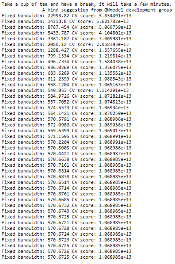
Results above show that:

• The CV score is becoming smaller and smaller.
• The recommended bandwidth is 570.6638 metres as it converged and stabilised here with the CV score of 1.068985e+13.

10.1.2 GWModel method - fixed bandwidth

gwr.fixed <- gwr.basic(formula = resale_price ~ floor_area_sqm + storey_order + remaining_lease_mths + PROX_CBD + PROX_ELDERLYCARE + PROX_HAWKER + PROX_MRT + PROX_PARK + PROX_MALL  + PROX_SUPERMARKET + WITHIN_350M_KINDERGARTEN + WITHIN_350M_CHILDCARE + WITHIN_350M_BUS + WITHIN_1KM_PRISCH, data=rs.sp, bw=bw.fixed, kernel = 'gaussian', longlat = FALSE)
gwr.fixed

Due to the long run time, the output of the above computation will be shown in the following screenshot:

Screenshot of gwr.fixed computation

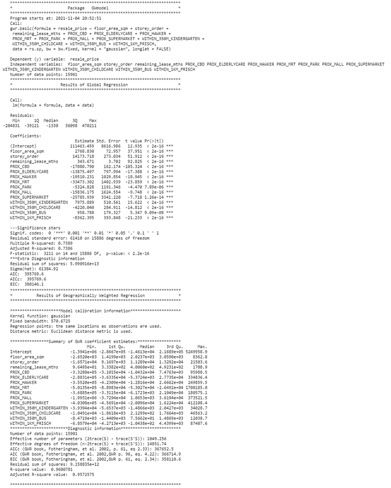
Great! :D Results above show that:

• The adjusted r-square of the GWR is 0.9572575 which is significantly better than the global multiple linear regression model of 0.7386.

10.2 Build Adaptive Bandwidth GWR Model

In this section, we will calibrate the gwr-based hedonic pricing model by using adaptive bandwidth approach.

10.2.1 Compute the adaptive bandwidth

• Similar to the earlier section, we will first use bw.ger() to determine the recommended data point to use.
• The code chunk used look very similar to the one used to compute the fixed bandwidth except the adaptive argument has changed to TRUE.

bw.adaptive <- bw.gwr(formula = resale_price ~ floor_area_sqm + storey_order + remaining_lease_mths + PROX_CBD + 
                        PROX_ELDERLYCARE + PROX_HAWKER + PROX_MRT + PROX_PARK + PROX_MALL  + PROX_SUPERMARKET  +
                        WITHIN_350M_KINDERGARTEN + WITHIN_350M_CHILDCARE + WITHIN_350M_BUS + WITHIN_1KM_PRISCH, 
                      data=rs.sp, approach="CV", kernel="gaussian", adaptive=TRUE, longlat=FALSE)

Due to the long run time, the output of the above computation will be shown in the following screenshot:

Screenshot of bw.adaptive computation

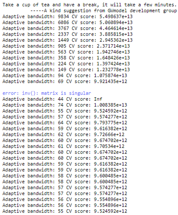
Results above show that:

• 55 is the recommended data points to be used

10.2.2 Construct the adaptive bandwidth GWR model

• Calibrate the GWR-based hedonic pricing model by using adaptive bandwidth and gaussian kernel

gwr.adaptive <- gwr.basic(formula = resale_price ~ floor_area_sqm + storey_order + remaining_lease_mths + PROX_CBD +
                            PROX_ELDERLYCARE + PROX_HAWKER + PROX_MRT + PROX_PARK + PROX_MALL + PROX_SUPERMARKET + 
                            WITHIN_350M_KINDERGARTEN + WITHIN_350M_CHILDCARE + WITHIN_350M_BUS + WITHIN_1KM_PRISCH, 
                          data=rs.sp, bw=bw.adaptive, kernel = 'gaussian', adaptive=TRUE, longlat = FALSE)
gwr.adaptive

Due to the long run time, the output of the above computation will be shown in the following screenshot:

Screenshot of gwr.adaptive computation

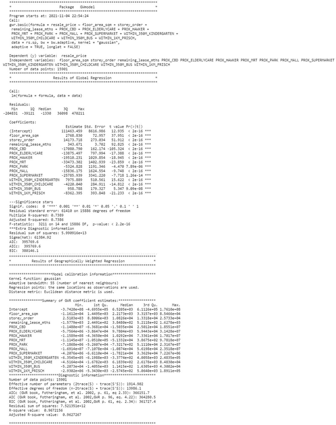
Results above show that:

• The adjusted r-square of the GWR is 0.9627267 which is significantly better than the global multiple linear regression model of 0.7386

Overall, we can see that the adaptive bandwidth GWR model has the best adjusted R-square value of 0.9627267 as compared to Multiple Linear Regression Model and Fixed Bandwidth GWR model. Hence, we will be using it to visualise GWR output in the next section.

11. Visualising GWR Output

In addition to regression residuals, the output feature class table includes fields such as:

• Condition Number: which evaluates local collinearity. In the presence of strong local collinearity, the results become unstable. Results associated with condition numbers larger than 30, may be unreliable.
• Local R2: values range between 0.0 and 1.0 which indicates how well the local regression model fits observed y values. Low values indicate the local model is performing poorly.
• Predicted: estimated (or fitted) y values computed by GWR.
• Residuals: to obtain the residual values, the fitted y values are subtracted from the observed y values. Standardized residuals have a mean of zero and a standard deviation of 1.
• Coefficient Standard Error: measures the reliability of each coefficient estimate. Confidence in those estimates are higher when standard errors are small in relation to the actual coefficient values. Large standard errors may indicate problems with local collinearity.

They are all stored in a SpatialPointsDataFrame or SpatialPolygonsDataFrame object integrated with fit.points, GWR coefficient estimates, y value, predicted values, coefficient standard errors and t-values in its “data” slot in an object called SDF of the output list.

11.1 Converting SDF into sf data.frame

• Here we use
  • st_as_sf() function of sf package to convert the data frame into sf object
  • st_transform() function of sf package to transform the coordinates of the sf object

rs.sf.adaptive <- st_as_sf(gwr.adaptive$SDF) %>%
  st_transform(crs=3414)

rs.sf.adaptive.svy21 <- st_transform(rs.sf.adaptive, 3414)
rs.sf.adaptive.svy21 

gwr.adaptive.output <- as.data.frame(gwr.adaptive$SDF)
rs.sf.adaptive <- cbind(rs.res.sf, as.matrix(gwr.adaptive.output))

glimpse(rs.sf.adaptive)

11.2 Write file to rds

• To avoid rerunning the above codes again, we can now save it as an rds file.

rs_adaptive_rds <- write_rds(rs.sf.adaptive, "data/aspatial/rds/rs_adaptive.rds")

11.3 Read rs_adaptive RDS file

Code Chunk

rs.sf.adaptive <- read_rds("data/aspatial/rds/rs_adaptive.rds")

Glimpse

glimpse(rs.sf.adaptive)

Rows: 15,901
Columns: 73
$ resale_price                <dbl> 330000, 360000, 370000, 375000, ~
$ floor_area_sqm              <dbl> 92, 91, 92, 99, 92, 92, 92, 92, ~
$ storey_order                <int> 1, 3, 1, 2, 2, 4, 3, 2, 4, 3, 3,~
$ remaining_lease_mths        <dbl> 684, 738, 733, 700, 715, 732, 70~
$ PROX_CBD                    <dbl> 8.824749, 9.841309, 9.560780, 9.~
$ PROX_ELDERLYCARE            <dbl> 0.2514065, 0.6318448, 1.0824168,~
$ PROX_HAWKER                 <dbl> 0.44182653, 0.26972560, 0.258295~
$ PROX_MRT                    <dbl> 0.6885144, 1.0969096, 0.8862859,~
$ PROX_PARK                   <dbl> 0.7450859, 0.4294870, 0.7800777,~
$ PROX_GOOD_PRISCH            <dbl> 1.2703931, 0.4045792, 2.0942375,~
$ PROX_MALL                   <dbl> 0.5534331, 1.0677012, 0.9751113,~
$ PROX_CHAS                   <dbl> 1.364596e-01, 2.569863e-01, 1.90~
$ PROX_SUPERMARKET            <dbl> 0.2708222, 0.3101889, 0.3187560,~
$ WITHIN_350M_KINDERGARTEN    <int> 1, 1, 1, 1, 1, 1, 1, 1, 1, 0, 1,~
$ WITHIN_350M_CHILDCARE       <int> 6, 5, 2, 3, 3, 2, 3, 4, 3, 2, 4,~
$ WITHIN_350M_BUS             <int> 8, 8, 8, 7, 6, 9, 6, 6, 5, 4, 10~
$ WITHIN_1KM_PRISCH           <int> 2, 2, 1, 2, 2, 1, 3, 2, 2, 2, 2,~
$ LOG_SELLING_PRICE           <dbl> 12.70685, 12.79386, 12.82126, 12~
$ MLR_RES                     <dbl> -53437.543, -31360.769, -20277.8~
$ Intercept                   <dbl> 450625.40, 219132.26, -239121.55~
$ floor_area_sqm.1            <dbl> 2663.8680, 1754.2820, 2803.2259,~
$ storey_order.1              <dbl> 19819.366, 17864.350, 9906.028, ~
$ remaining_lease_mths.1      <dbl> 478.4616, 457.5624, 710.7935, 43~
$ PROX_CBD.1                  <dbl> -70930.226, -36578.084, -3966.53~
$ PROX_ELDERLYCARE.1          <dbl> 12961.930, -4052.943, -66619.714~
$ PROX_HAWKER.1               <dbl> 7663.184, 45314.821, -29691.697,~
$ PROX_MRT.1                  <dbl> 22162.794, -30945.094, -49355.92~
$ PROX_PARK.1                 <dbl> -55468.7722, 575.8611, -120109.6~
$ PROX_MALL.1                 <dbl> -128317.494, -6778.338, 73384.44~
$ PROX_SUPERMARKET.1          <dbl> 13783.2095, 49272.2268, -36668.9~
$ WITHIN_350M_KINDERGARTEN.1  <dbl> 86.70467, 7756.08521, -4572.7501~
$ WITHIN_350M_CHILDCARE.1     <dbl> -1209.78379, 2853.12224, 1344.87~
$ WITHIN_350M_BUS.1           <dbl> 7386.4498, -28.9138, 2688.6847, ~
$ WITHIN_1KM_PRISCH.1         <dbl> -6821.190, -15341.235, -15594.72~
$ y                           <dbl> 330000, 360000, 370000, 375000, ~
$ yhat                        <dbl> 368416.7, 385189.2, 358453.1, 37~
$ residual                    <dbl> -38416.6907, -25189.2454, 11546.~
$ CV_Score                    <dbl> 0, 0, 0, 0, 0, 0, 0, 0, 0, 0, 0,~
$ Stud_residual               <dbl> -1.82540375, -1.13376401, 0.5298~
$ Intercept_SE                <dbl> 174303.86, 97699.33, 162199.65, ~
$ floor_area_sqm_SE           <dbl> 499.3217, 378.3388, 856.0818, 35~
$ storey_order_SE             <dbl> 1180.0127, 1550.9533, 1211.1528,~
$ remaining_lease_mths_SE     <dbl> 16.10308, 19.50918, 23.78930, 16~
$ PROX_CBD_SE                 <dbl> 18035.787, 8037.991, 13797.135, ~
$ PROX_ELDERLYCARE_SE         <dbl> 33814.032, 12456.030, 20628.228,~
$ PROX_HAWKER_SE              <dbl> 26418.654, 19268.193, 28094.306,~
$ PROX_MRT_SE                 <dbl> 40535.942, 16205.349, 26328.027,~
$ PROX_PARK_SE                <dbl> 21702.581, 19534.332, 36724.222,~
$ PROX_MALL_SE                <dbl> 55299.92, 19602.18, 28241.86, 15~
$ PROX_SUPERMARKET_SE         <dbl> 37832.59, 24775.42, 23846.11, 22~
$ WITHIN_350M_KINDERGARTEN_SE <dbl> 4997.913, 4183.356, 6023.687, 37~
$ WITHIN_350M_CHILDCARE_SE    <dbl> 2473.156, 1381.719, 2653.410, 13~
$ WITHIN_350M_BUS_SE          <dbl> 1524.4901, 1291.9383, 1595.1020,~
$ WITHIN_1KM_PRISCH_SE        <dbl> 5996.636, 4676.567, 6259.941, 41~
$ Intercept_TV                <dbl> 2.5852864, 2.2429250, -1.4742421~
$ floor_area_sqm_TV           <dbl> 5.3349730, 4.6368020, 3.2744836,~
$ storey_order_TV             <dbl> 16.795892, 11.518303, 8.179007, ~
$ remaining_lease_mths_TV     <dbl> 29.712429, 23.453699, 29.878704,~
$ PROX_CBD_TV                 <dbl> -3.9327492, -4.5506502, -0.28749~
$ PROX_ELDERLYCARE_TV         <dbl> 0.38332990, -0.32537997, -3.2295~
$ PROX_HAWKER_TV              <dbl> 0.29006717, 2.35179402, -1.05685~
$ PROX_MRT_TV                 <dbl> 0.54674427, -1.90956051, -1.8746~
$ PROX_PARK_TV                <dbl> -2.55586060, 0.02947944, -3.2705~
$ PROX_MALL_TV                <dbl> -2.3203919, -0.3457951, 2.598428~
$ PROX_SUPERMARKET_TV         <dbl> 0.36432106, 1.98875483, -1.53773~
$ WITHIN_350M_KINDERGARTEN_TV <dbl> 0.01734817, 1.85403442, -0.75912~
$ WITHIN_350M_CHILDCARE_TV    <dbl> -0.4891660, 2.0649074, 0.5068476~
$ WITHIN_350M_BUS_TV          <dbl> 4.84519377, -0.02238017, 1.68558~
$ WITHIN_1KM_PRISCH_TV        <dbl> -1.1375029, -3.2804482, -2.49119~
$ Local_R2                    <dbl> 0.9112596, 0.8650748, 0.9767927,~
$ coords.x1                   <dbl> 29179.92, 28423.42, 30550.38, 28~
$ coords.x2                   <dbl> 38822.08, 39745.94, 39588.77, 39~
$ geometry                    <POINT [m]> POINT (29179.92 38822.08),~

11.4 Summary statistics of y and yhat

The following code chunk checks the statistics of the observed and the predicted resale price values, y and yhat, using summary() function of base R package.

Summary of Observed

summary(rs.sf.adaptive$y)

   Min. 1st Qu.  Median    Mean 3rd Qu.    Max. 
 218000  353000  405000  433589  470000 1186888 

Summary of Predicted

summary(rs.sf.adaptive$yhat)

   Min. 1st Qu.  Median    Mean 3rd Qu.    Max. 
 229563  355021  403826  433315  468740 1067918 

• Range, interquartile range, and standard deviation are the 3 commonly used measures of dispersion.
• From the summary statistics of the predicted resale prices above, we can see that:
  • For range,
    • The lowest predicted price for 4-room hdb flat is $229,563 while the highest predicted price is $1,067,918.
    • Since the range is quite large, we can say that there is high variablity in the dataset.
    • However, since the range is easily influenced by outliers, it can’t tell us about the shape of the distribution of values on its own.
  • For interquartile range,
    • It gives us the range of the middle half of a dataset.
    • Here, the predicted resale price for Q3 is farther away from the predicted median price than Q1 is from the predicted median price.
    • Hence, we can say that there is a greater dispersion among the larger values of predicted resale prices than among the smaller values of predicted resale price.
  • Since our median is less than our mean, we can also say that the distribution of our predicted resale prices are skewed to the right.
• The summary statistics of the observed and predicted resale prices are similar in terms of the observations above as well since the numbers only differ by a few thousands (3 to 10).

11.5 Visualising Local R2

tmap_mode("view")
tm_shape(mpsz_sf) +  
  tm_polygons(alpha = 0.1) +
  tm_shape(rs.sf.adaptive) +  
  tm_dots(col = "Local_R2",
          border.col = "gray60",
          border.lwd = 1) +
  tm_view(set.zoom.limits = c(11,14)) +
tm_basemap("OpenStreetMap")

tmap_mode("plot")

• Results above show that:
  • A few HDBs in the North-East and East region are in a lighter shade which implies that the GWR model is unable to predict well in these areas.
  • However, most of the Local_R2 values are within 0.8 to 1.0 indicated by the darker shade of orange.
  • Thus, we can conclude that the 4-room HDB resales prices can be explained well by the adaptive GWR model.

11.6 Visualizing Observed and Predicted Y

The following code chunk will spatial point maps of the Observed and Predicted Y values using tmap package for comparison.

actual <- tm_shape(mpsz_sf)+
          tm_polygons() +
          tmap_options(check.and.fix = TRUE) +
        tm_shape(rs.sf.adaptive) +  
          tm_dots(col = "y",
                  border.col = "gray60",
                  border.lwd = 1) +
        tm_layout(title="Actual Y")

predicted <- tm_shape(mpsz_sf)+
              tm_polygons() +
              tmap_options(check.and.fix = TRUE) +
            tm_shape(rs.sf.adaptive) +  
              tm_dots(col = "yhat",
                      border.col = "gray60",
                      border.lwd = 1) +
        tm_layout(title="Predicted Y")
        
tmap_arrange(actual, predicted)

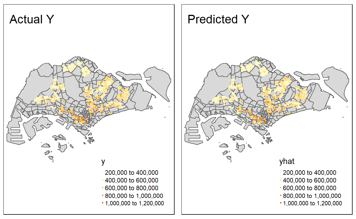
From the above plots, we can see that it looks roughly the same which means that the prediction done by the adaptive GWR model is good.

12. Conclusion

To conclude, the hedonic pricing model is the best model as it is able to explain the highest percentage, about 96%, of four-room HDB resale prices transacted from 1st January 2019 to 30th September 2020.

The final explanatory variables used that contributed to this high percentage are:

• Structural Factors like:
  • Floor area
  • Remaining lease
  • Storey range
• Locational Factors like:
  • Proximity to CBD
  • Proximity to Elderlycare
  • Proximity to Hawker
  • Proximity to MRT
  • Proximity to Park
  • Proximity to Shopping Malls
  • Proximity to Supermarkets
  • Number of Kindergartens within 350 metres
  • Number of Childcare within 350 metres
  • Number of Bus stops within 350 metres
  • Number of Primary Schools within 1 kilometres

References

• Categorical variables
• Categorical variables in regression
• IQR
• Hands-on Exercise 9: Calibrating Hedonic Pricing Model for Private Highrise Property with GWR Method by Prof Kam